Chapter 5 Bayesian Inference – Update Beliefs
- Probability is interpreted as confidence in a hypothesis.
- Model parameters are random variables which have prior (before data) and posterior distributions (after data).
- Estimating models means updating the distributions of the parameters.
- A statistical modeling mindset with frequentism and likelihoodism as alternatives.
A Bayesian walks into a bar and asks for a beer. The bartender says “You’re not allowed to drink here.” The Bayesian looks around the bar and sees that there are no other customers, so he asks “Why not? Is it because I’m a Bayesian?” The bartender replies “Yes, we don’t allow Bayesians in here.” The Bayesian is about to leave, but then he asks “What would happen if I came in here and told you that I’m not a Bayesian?” The bartender would reply “That’s impossible, everyone is a Bayesian.”
People teaching Bayesian statistics usually start with Bayes’ theorem. Or for a more philosophical twist, they start with the Bayesian interpretation of probability as “degree of belief”. But there is one Bayesian premise, from which the entire Bayesian mindset unfolds:
Model parameters are random variables.
The mean of a distribution, a coefficient in a logistic regression model and the correlation coefficient – all these parameters are random variables and have a distribution.
Let’s follow the implications of the parameters-are-variables premise to its full conclusion.
- Parameters are random variables.
- Modeling goal: estimate parameter distribution, given the data (posterior).
- But there is a problem: P(parameters | data) is unnatural to estimate.
- Fortunately, there is a mathematical “trick”, the Bayes’ theorem.
- The theorem inverses the condition to P(data | parameters). The good old likelihood.
- Bayes’ theorem also involves P(parameters) the priori distribution.
- That’s why Bayesians must specify a parameter distribution before observing data.
- Model estimation equals a belief update: priori \(\rightarrow\) posterior.
And all that from the assumption that parameters are variables too. But that’s not all. There are implications that I left out. Let’s go deeper, and this time I’ll start with Bayes’ theorem.
Bayesians want to learn the distribution of the model parameters given the data. To make this posterior distribution P(parameters | data) computable, Bayesians use a trick that earned them their name: the Bayes’ theorem. Bayes’ theorem inverts the conditional probability: posterior = (likelihood x prior) / evidence. Forget about the evidence right away, since the term is intractable in most cases. As a workaround Bayesians use other techniques (Monte Carlo sampling) to get the posterior distribution, but we will get to that later. The prior is the probability distribution of the parameter before taking any data into account. The priori is “updated” by multiplying it by the data likelihood. The result is the posterior probability distribution, an updated belief about the parameters (Figure 5.1)
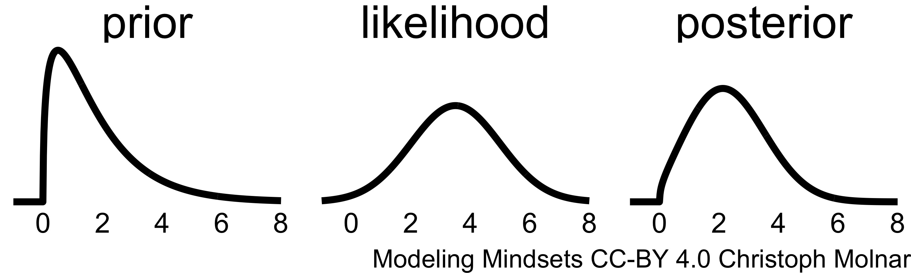
FIGURE 5.1: The posterior distribution (right) is the scaled product of prior and likelihood.
5.1 Bayes’ Theorem Demands A Prior
Bayesians assume that parameters have a prior probability distribution. Priors are a consequence of saying that parameters are random variables, and a technical requirement for working with the Bayes’ theorem.
But how can Bayesians know the distribution of parameters before observing any data? Like, what’s the prior distribution of a parameter in logistic regression that models the effect of alcohol on diabetes? Many considerations go into the choice of a prior.
The first consideration in choosing a prior is the parameter space, which is the set or range of values that the parameters can take on. For examples can the parameter only take on positive values? Then the prior must have a probability of zero for negative values, for example, the Gamma distribution.
The Bayesian can encode further domain knowledge with the prior. If the data follow a Binomial distribution (say number of tails in coin tosses), the Beta distribution is a possible prior for the success probability parameter (see Figure 5.2). The Beta distribution itself has parameters which the modeler has to specify. Another chance to instill domain knowledge: Any prior information about success probability can be used. Maybe there is reason to expect the parameter to be symmetrically distributed around 0.5, with 0 and 1 being rather unlikely. This would make sense for coin tosses. Or maybe the parameter is lower, around 0.25? There is even a Beta prior that puts the greatest probability symmetrically on 0 and 1.
Without domain knowledge about the parameter, the modeler can use “uninformative” or “objective” priors (Yang and Berger 1996). Uninformative priors may produce results identical or similar to those of frequentist inference (for example for credible intervals). However, objective priors are not always as objective as they might seem and are not always easy to come by.
Another factor influencing the choice of prior is mathematical convenience: Conjugate priors remain in the same family of distributions when multiplied by the right likelihood functions, allowing to derive the posterior distribution analytically – a big plus before improvements in computational resources shook up the Bayesian landscape.
Critics of the Bayesian mindset decry that the choice of a prior is subjective. [^objective-priors] Bayesians might also be annoyed having to pick priors, especially if the model has many parameters and the prior choice is not obvious. But while priors can be seen a problem, they can also be a solution:
- priors can regularize the model, especially if data are scarce
- priors can encode domain knowledge and prior experimental results
- priors allows a natural handling of measurement errors and missing data.
The prior gives Bayesian modeling all this flexibility.
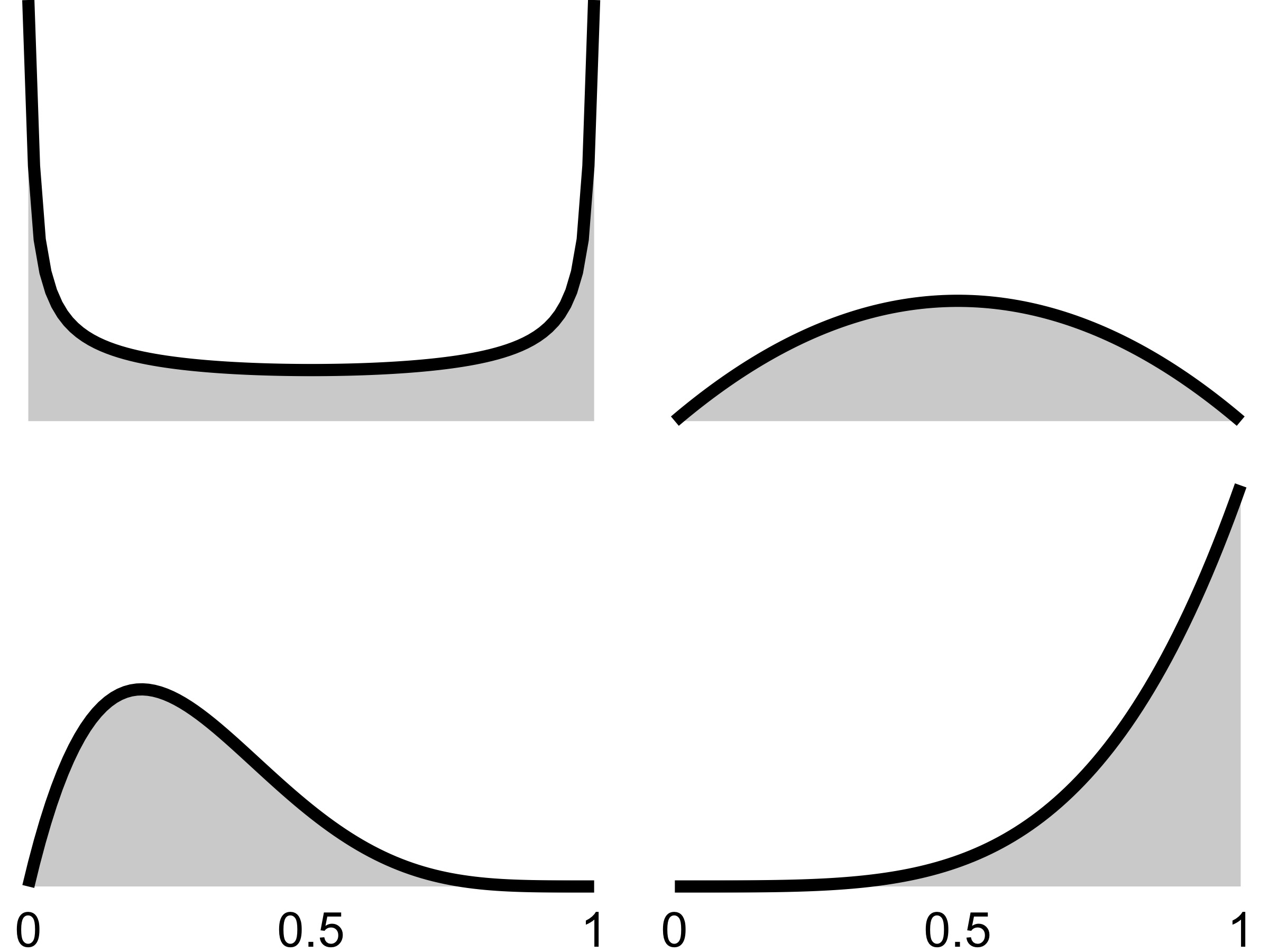
FIGURE 5.2: Various Beta prior distributions for the success probability in a Binomial distribution.
Fun fact: Bayesian models can, in theory, already be used, for example for making prediction.5 But that wouldn’t be the best idea, and instead Bayesians update the prior using data, or to be more specific, using the likelihood function.
5.2 The Likelihood Unites All Statistical Mindsets
Prior aside, Bayesians make assumptions about the data distribution to specify the likelihood function P(data | theta), same as frequentists and likelihoodists. Discussions often focus on the differences between the mindsets, but at the core the 3 mindsets all use the likelihood. Especially in cases with a lot of data, models from different statistical mindsets will result in similar models. However, comparisons often focus on the use of priors or other differences. The more data is available, the more certain the likelihood becomes and the impact of the prior vanishes. What remains is how results may be interpreted, but the conclusions will be similar: With enough data, a frequentist coefficient that is significantly different from 0 will likely show a posterior distribution with little mass on 0.
While frequentists and likelihoodists get their inference mostly from the likelihood function, Bayesians want the posterior.
5.3 The Ultimate Goal: The Posterior
The goal of the Bayesian modelers is to estimate the posterior distributions of the parameters. Once the modelers have the posteriors, they can interpret them, make predictions, and draw conclusions about the world.
In the ideal case, the posterior can be written down as an explicit formula and computed directly. But that’s rarely the case (only for certain priors). And for most Bayesian models it’s impossible to obtain a closed form of the posterior. The problem is the evidence term in the Bayes’ theorem: it’s usually unfeasible to compute.
Fortunately Bayesians have a way out: Instead of computing the posterior, they sample from it. Approaches such as Markov Chain Monte Carlo (MCMC) and derivations thereof are used to generate samples from the posterior distribution. The rough idea of MCMC and similar approaches is as follows: Start with some initial (random) values for the parameters. Then multiple cycles of: Propose new parameter values, either accept or reject them, if accepted continue with these parameters. MCMC has many variants with different proposal and acceptance functions that ensure that samples converge to the posterior distribution. One MCMC run produces a “chain” of samples from the posterior distribution. Multiple MCMC runs produce multiple chains. The intuition behind this procedure: A chain is a random walk through the posterior, “visiting” regions with a large posterior proportionally more often. That’s why samples can be seen as samples from the posterior.
While this sampling sounds very tedious, most Bayesian modeling software can run MCMC automatically. But it can be slow, especially compared to frequentist maximum likelihood procedures. A quicker but heuristic alternative is variational inference.(Blei et al. 2017)
The posterior samples can be visualized with a histogram or a density estimator for a smoother looking curve. Visualizing the entire posterior is the most informative way of reporting the Bayesian results.
5.4 All Information Is In The Posterior
The posterior distributions contain everything that the models learned from the data. Visualizing the posteriors provides provides access to that full information. But people are fans of numbers and tables as well: the fewer and simpler, the better. While some argue not to summarize the posterior (Tiao and Box 1973), many modelers do it anyways and it can provide a good summary. Any method that describes distributions can be used. Some examples:
- The parameter value with the highest posterior probability.
- Probability that the parameter is >10: Integrate the posterior from 10 to infinity.
- 95% credible interval: range from the 2.5% and the 97.5% quantile.
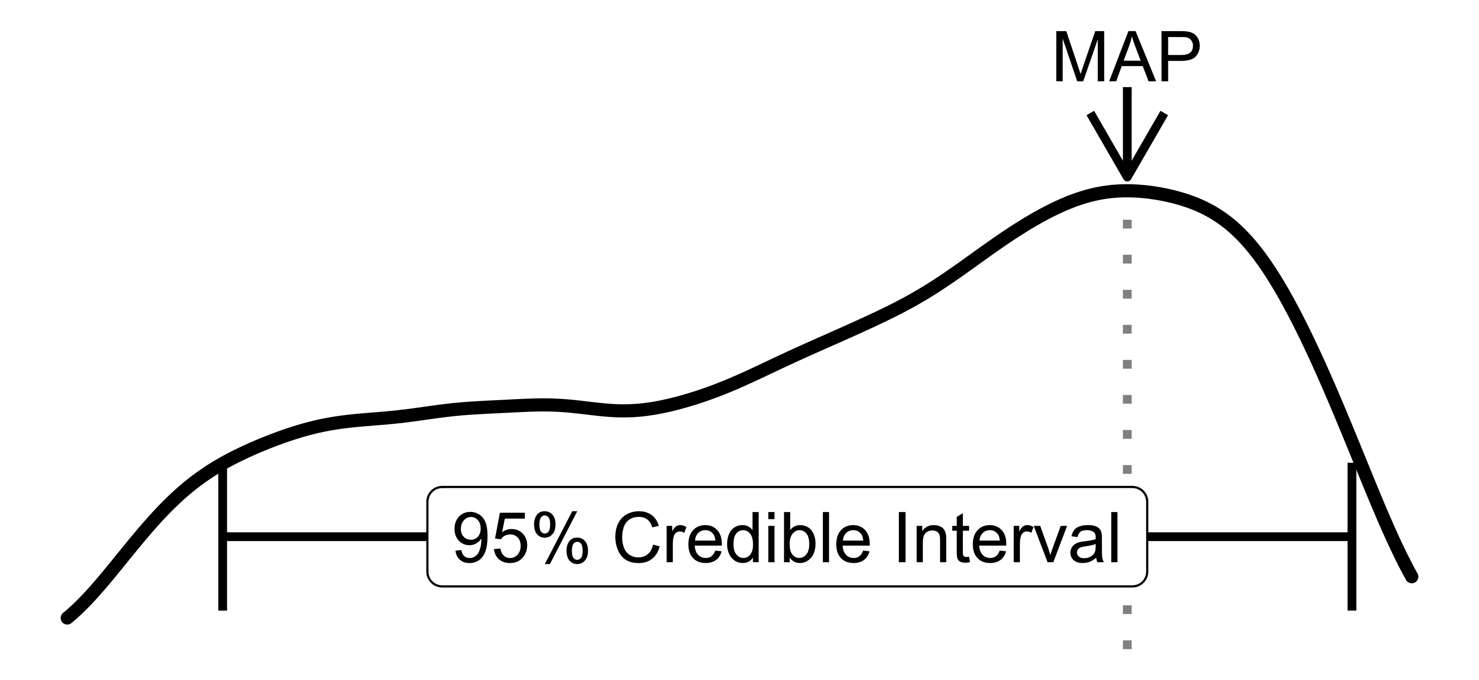
FIGURE 5.3: Describing the posterior distribution with the 95% credibility interval and the maximum a posteriori estimation (MAP).
5.5 From Model to World
Like in the other statistical modeling mindsets, Bayesians build statistical models to approximate the data-generating process with probability distributions. These distributions are parameterized, and Bayesians say that these parameters are themselves random variables. Learning from data means updating the model parameters. But after the “update” there is no definite answer on what the true parameters are. Instead, the modeler was able to improve the information about the parameter distributions. But the posterior doesn’t encode uncertainty inherent in nature, as in quantum mechanics. Instead, the posterior expresses the uncertainty of information about the parameters. That’s different from how frequentists connect their statistical models to the world. Frequentists assume that there are some unknown but fixed parameters that can be approximated with statistical models. Uncertainty is a function of the estimators, and conclusions about the world are derived from how these estimators are expected to behave when samples and experiments are repeated.
Another consequence of parameters being random variables: To predict, the Bayesian must simulate. Because if parameters are random variables, so are the predictions. Prediction means: sample parameters from the posteriors, then predict with the model. Repeat multiple times and average the results. The uncertainty of the parameters propagates into uncertainty of predictions. And if that seems inconvenient at first glance, it’s much more honest and informative than a point estimate on the second glance. Uncertainty is a natural part of Bayesian modeling.
5.6 Strengths
- Bayesian models can leverage prior information such as domain knowledge.
- Bayesian inference provides an expressive language to build models that naturally propagate uncertainty. This makes it easy to work with hierarchical data, measurement errors and missing data.
- Bayesian interpretation of probability is arguably more intuitive than frequentist interpretation: When practitioners misinterpret frequentist confidence intervals, it’s often because they interpret them as credible intervals.
- Bayesian inference decouples inference (estimate posterior) and decision making (draw conclusions from posterior). Frequentists hypothesis tests entangle inference and decision making.
- Bayesian statistics adheres to the likelihood principle: all the evidence from the data is contained in the likelihood function.
- General benefit: Bayesian updating as a mental model for how we update our own beliefs about the world.
References
This is called the prior predictive simulation and is used to check that the chosen priors produce reasonable data. The modeler simulates by first sampling parameters from the priors and using those parameters to generate data. Repeating this several times results in a distribution of data.↩︎