Chapter 3 Statistical Modeling – Reason Under Uncertainty
- The world is best described with probability distributions.
- Statisticians estimate models to learn aspects of distributions from data.
- Model parameters are interpreted to reason about the real world.
- Additional assumptions needed to draw conclusion: frequentism inference, Bayesian inference or likelihoodism.
- Machine learning is an alternative mindset.
The statistician had come to duel the monster of randomness. The fight was fierce and the statistician was driven back, step by step. But with every attack, the statistician learned more about the monster. Suddenly the statistician realized how to win: figure out the data-generating process of the monster. With one final punch, the statistician separated signal from randomness.
Do you become more productive when you drink a lot of water? Your productivity will vary naturally from day to day – independent of your water intake. This uncertainty makes it difficult to express productivity as a function of water intake. Many questions are subject to randomness, making it difficult to see the signal and separate it from the noise.
Statistical modeling provides a mindset and mathematical tools to handle uncertainty:
- Assumption: data are generated by a process that involves probability distributions.
- Statisticians replicate this process with statistical models.
- Statistical models target aspects of these (assumed) distributions and are estimated with data.
- Statisticians interpret the model (parameters) to reason under uncertainty.
Let’s talk about the elementary units in statistical modeling: the random variable.
3.1 Every “Thing” Is A Random Variable
Statisticians think in random variables: mathematical objects that encode uncertainty in the form of probability distributions. In statistical modeling, data are realizations of random variables (see Figure 3.1). If someone drank 2.5 liters of water, that is a realization of the random variable “daily water intake”. Other random variables:
- Outcome of a dice roll.
- Monthly sales of an ice cream truck.
- Whether or not a customer has canceled their contract last month.
- Daily amount of rain in Europe.
- Pain level of patients arriving at the emergency room.
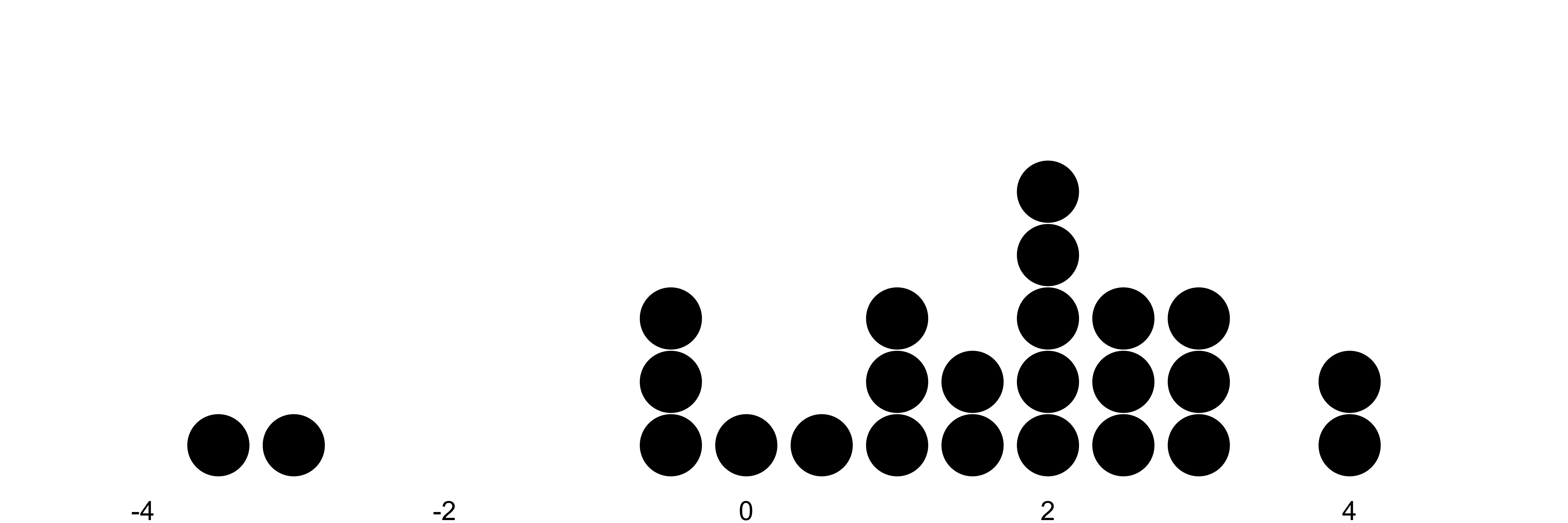
FIGURE 3.1: Each dot represents a data point, a realizations of a random variable. The x-axis shows the value of the variable. Dots are stacked up for frequently occurring values.
Probability distributions describe how variables “behave”. A distribution is a function that gives each possible outcome of a variable a probability. Value in, probability out. For the outcome of a fair dice, there are 6 possible outcomes, each with a probability of 1/6. For non-discrete outcomes such as monthly sales, the Normal distribution is a common choice, see Figure 3.2 on the left. There is huge arsenal of probability distributions: The Normal distribution, the Binomial distribution, the Poisson distribution, … The goal in statistical modeling is to pick the distributions that best match the nature of the variables.
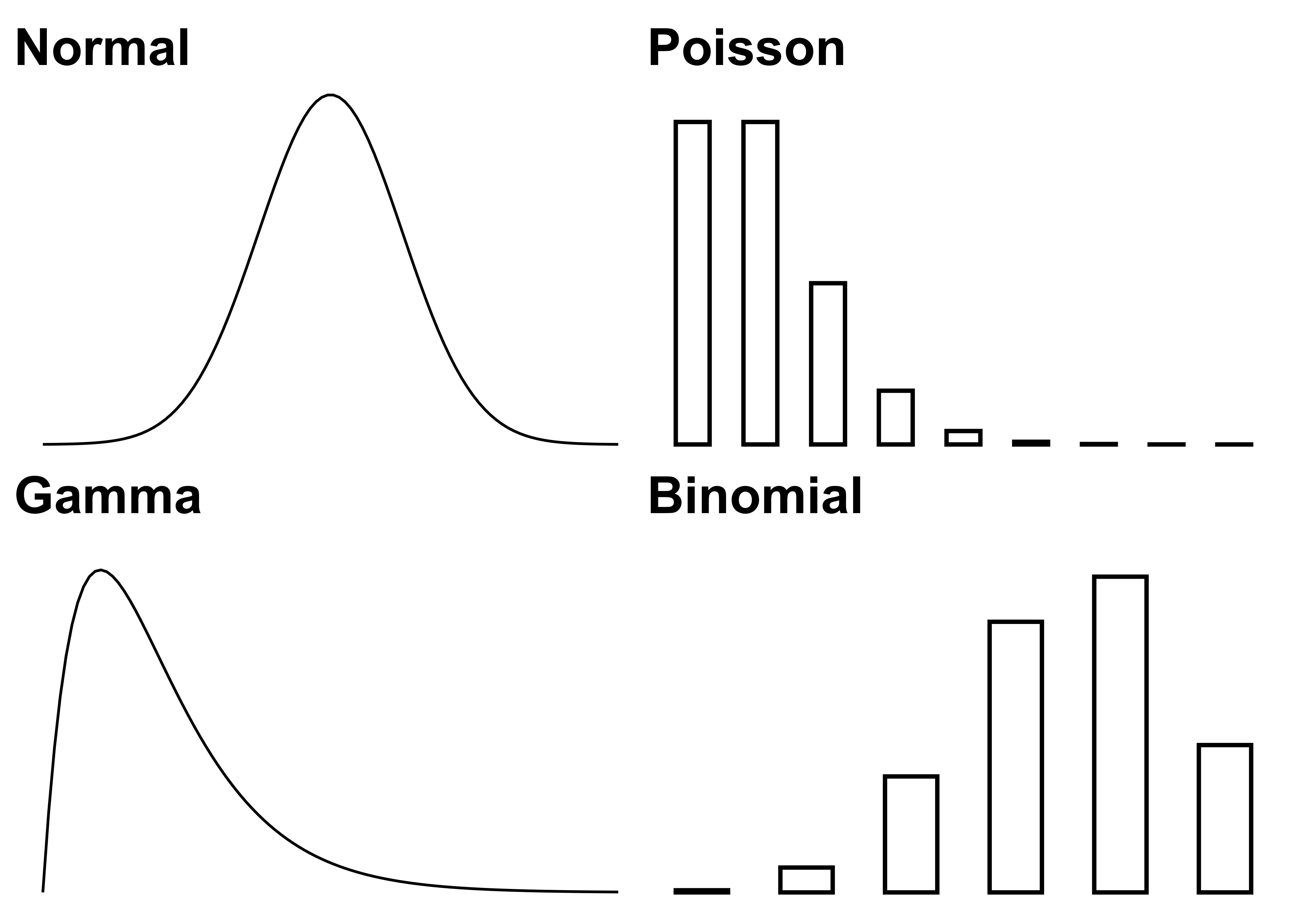
FIGURE 3.2: Distributions
Statisticians think deeply about the data-generating process. It’s part of the mindset, a natural consequence of contemplating distributions and assumptions about the data. This focus stands in contrast with machine learning, where solving the task at hand (like prediction) is more important than replicating some data-generating process.
But probability distributions only exist in an abstract, mathematical realm. Statistical models connect these theoretic distributions with the data.
3.2 Models Connect Theory And Data
Statistical models have a fixed and a flexible part. In the fixed part are all the assumptions that were made about how the data were generated, such as the assumed distributions. Statistical models target aspects of a distribution such as:
- Conditional mean, typically estimated with regression models such as linear regression.
- The probability of an outcome conditional on other variables, for example, estimated with logistic regression.
- Quantiles of a numerical outcome, estimated with quantile regression.
- The full distribution, with Gaussian mixture models as a possible estimator.2
- The mean of a distribution, estimated with a simple average.
These aspects of the distribution like the conditional mean, are usually represented through model parameters. Model parameters are the “flexible” part of the model. Statisticians “fit” models by optimizing the parameter so that the data seem likely under the statistical model. In many cases, the likelihood function is used to measure how likely a data observation is given a certain value for a model parameter. That’s a classic optimization problem: Maximize the likelihood function with respect to the parameters. Statisticians use optimization methods such as gradient-based methods or more sophisticated optimization such as the expectation-maximization algorithm. For cases such as linear regression it’s even possible to have an explicit solution.
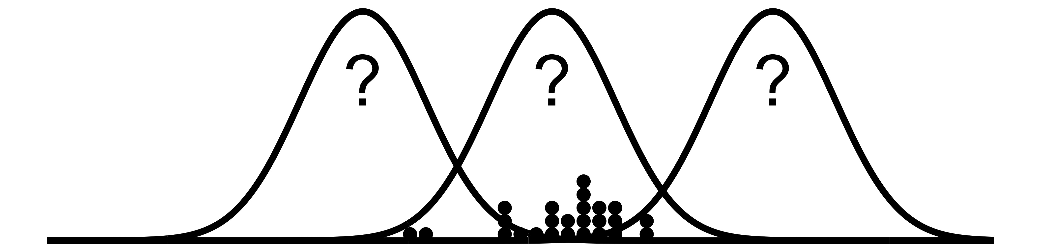
FIGURE 3.3: Fitting distributions to data
Model parameters are not only tuning knobs: Statisticians often draw conclusions from the parameter about real-world phenomena. This requires elementary representation: All relevant parts of the data-generating process are represented within the model as variables, parameters or functions. Interpretation of the statistical model, especially the estimated parameters is usually even more important to the statistician than prediction. And thanks to the elementary representation, these parameters reflect the data-generation process: the parameters contain information about the interesting aspects of the data distribution. For example, a positive model parameter means that increasing the value of the associated variable increases the predicted target.
3.3 Statisticians Diagnose Models
The evaluation of statistical models consists of two parts: model diagnostics and goodness-of-fit.
The role of model diagnostics is to check whether the modeling assumptions were reasonable. If the statistician assumes that a variable follows a Normal distribution, they can check this assumption visually. For example, with a Q-Q plot. Another assumption is homoscedasticity: The variance of the target is independent of other variables. Homoscedasticity can be checked visually by plotting the residuals (actual target minus its predicted value) against each of the other variables.
A model that passes these diagnostics is not automatically a good model.
Statisticians use goodness-of-fit measures to compare models and evaluate modeling choices, such as which variables to have in the model.
Typical goodness-of-fit measures are (adjusted) R-squared, Akaikes Information Criterion (AIC), the Bayes factor, and likelihood ratios.
Goodness-of-fit is literally a measure of how well the model fits the data.
Goodness-of-fit can guide the model building process and help decide which model to choose.
Goodness-of-fit is often computed with the same data that were used for fitting the statistical models. This choice may look like a minor detail, but it says a lot about the statistical modeling mindset. The critical factor here is overfitting: The more flexible a model is, the better it adapts to ALL the randomness in the data instead of learning patterns that generalize. Many goodness-of-fit metrics therefore account for model complexity, like the AIC or adjusted R-squared. Compare this to supervised machine learning: in this mindset, there is a strict requirement to always use “fresh” data for evaluation.
3.4 Drawing Conclusions About the World
Statistical models are built to make a decision, to better understand some property of the world, or to make a prediction. But using the model as a representation of the world isn’t for free. The statistician must consider the representativeness of the data and choose a mindset that allows the findings of the model to be applied to the world.
Considering the data-generating process also means thinking about the representativeness of the data, and thus the model. Are the data a good sample and representative of the quantity of the world the statistician is interested in? Let’s say a statistical modeler analyzes data on whether a sepsis screening tool successfully reduced the incidence of sepsis in a hospital. They conclude that the sepsis screening tool has helped reduce sepsis-related deaths at that hospital. Are the data representative of all hospitals in the region, the country, or even the world? Are the data even representative of all patients at the hospital, or are data only available from patients in intensive care unit? A good statistical modeler defines and discusses the “population” from which the data are a sample of.
More philosophical is the modeler’s attitude toward causality, the nature of probability, and the likelihood principle.
“It is unanimously agreed that statistics depends somehow on probability. But, as to what probability is and how it is connected with statistics, there has seldom been such complete disagreement and breakdown of communication since the Tower of Babel.”
– Leonard Savage, 19723
Statistical modeling is the foundation for learning from data. But we need another mindset on top of that to make the models useful.
- Frequentist inference sees probability as relative frequencies of events in long-run experiments.
- Bayesian inference is based on an interpretation of probability as a degree belief about the world.
- Likelihoodism equates the likelihood statistical models as evidence for a hypothesis.
3.5 Strengths
- Probability distribution and statistical models provide a language to describe the world and its uncertainties. The same language is often used in machine learning research to describe and understand machine learning algorithms.
- Statistical modeling has an extensive theoretical foundation: From measurement theory as the basis of probability to thousands of papers for specific statistical models.
- The data-generating process is a powerful mental model that encourages asking questions about the data.
- Conditional probability models can be used not only to learn about the parameters of interest, but also to make predictions.
- Probability distributions provides a language to express uncertainty. Bayesianism arguably has the most principled focus on formalizing and modeling uncertainty.
- Statistical models provide the means to reason under uncertainty.
3.6 Limitations
- The statistical modeling mindset struggles with complex distributions, like image and text data. This is where machine learning and especially deep learning shine.
- Modeling the data-generating process can be quite manual and tedious, as many assumptions have to be made. More automatable mindsets such as supervised learning are more convenient.
- Statistical models require many assumptions. Common assumptions: homoscedasticity, independent and identically distributed data (IID), linearity, independence of errors, lack of (perfect) multicollinearity, … Many statistical models were invented specifically to address possible violations of such assumptions, often coming with a price: more complexity, less interpretability.
- High goodness-of-fit doesn’t guarantee high predictive performance on test data. Statistical models often have inferior predictive performance than more complex models such as random forests. To be fair, this requires a supervised learning mindset evaluation.
Why would a statistician not always model the full distribution of the data, but often opts to simpler parts such as the conditional mean? Estimating the full distribution is usually more complex or requires making simplifying assumptions. Often the question doesn’t require the full distribution but can be answered with, for example, a conditional mean. Like the question of a treatment effect on a disease outcome.↩︎
Savage, Leonard J. The foundations of statistics. Courier Corporation, 1972.↩︎