Chapter 7 Causal Inference – What If
- Causal models place variables into cause-and-effect relationships.
- A model is a good generalization of the world if it encodes causality.
- Causal inference is not a stand-alone modeling mindset, but causal models are either integrated or translated into a statistical or machine learning models.
10-minute course on causality for old-school statisticians, says the note on the door. You can hear people chanting. “Correlation does not imply causation. Correlation does not imply causation, …”
Some time ago, I worked with a rheumatologist on the following question for axial spondyloarthritis, a chronic condition associated with inflammation of the spine. Does a type of drug, TNF-alpha blockers, reduce problematic bone formation the spine (ossification)? Infusion or injection of the blockers are great for reducing inflammation. Therefore it would be unethical to withhold the drugs in a clinical trial. The next best option for studying the drug effect on ossification: a statistical model with observational data. To predict ossification, the model included several variables such as patient age, disease duration, inflammation levels, medication, etc. The intermediate analysis showed that the drug didn’t reduce ossification.
By coincidence, the senior statistician of the patient registry attended a course on causal inference at about the same time. Applying what she had learned, she identified a flaw in the model: Inflammation was a potential mediator of the effect of TNF-alpha blockers on long-term ossification (see 7.1).
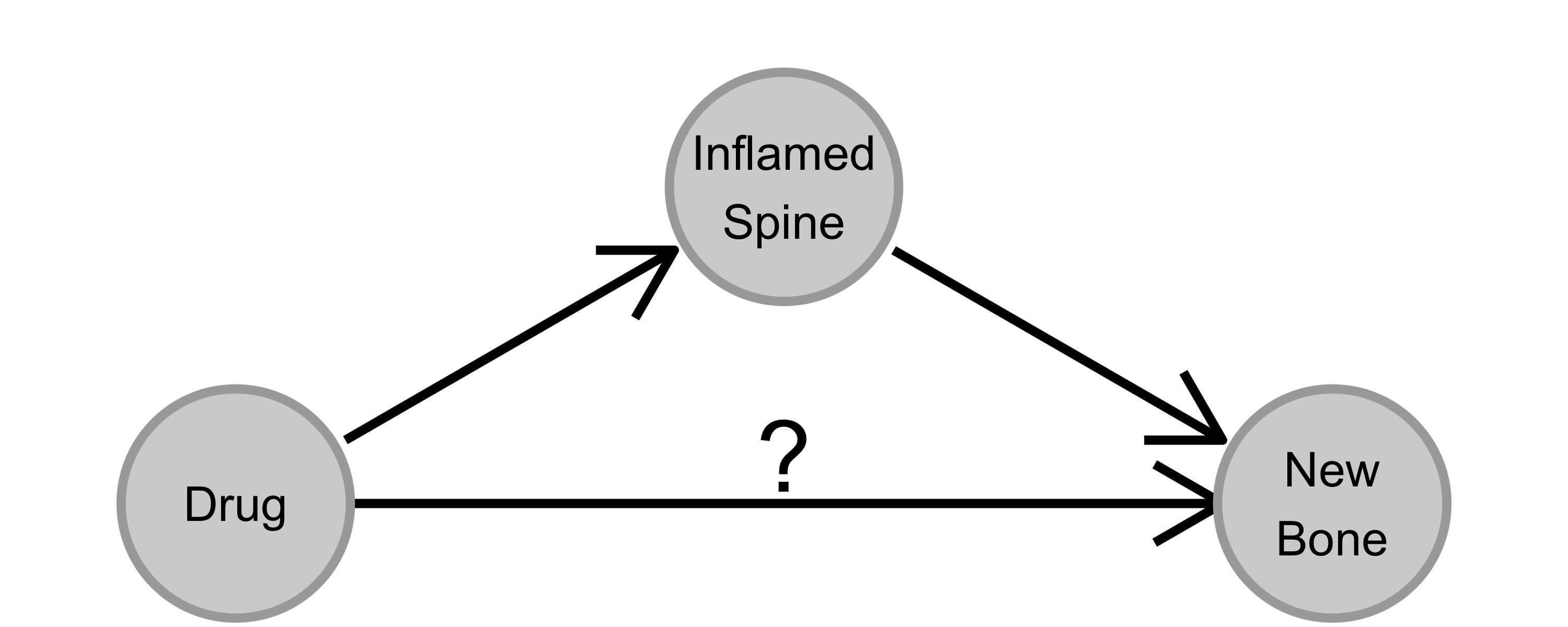
FIGURE 7.1: The drug was known to influence (reduce) inflammation. Inflammation was thought to cause ossification (new bone formation). The drug can, in theory, reduce ossification in two ways: directly, or indirectly via reducing inflammation.
The effect of the drug can be divided into a direct and an indirect effect. The total effect is the direct effect of the drug plus any indirect effects, in this case via reducing inflammation. We were interested in the total effect of the drug, but how we had specified the model, the coefficient for the drug had to be interpreted as direct effect. The indirect effect was fully reflected by the coefficient for the inflammation level (measured after start of medication). We therefore removed the inflammation variable7 and did a mediator analysis. After removal, the coefficient for the drug could be interpreted as total effect. The model then clearly showed that TNF-alpha blockers reduce ossification via reducing inflammation levels. It feels like common sense to me in hindsight, but not having a causal inference mindset at the time, I was thunderstruck.
7.1 Causality Not Always Part Of Statistical Modeling
I guess we all have an intuition about causality. Rain is a cause of a wet lawn. A drug can be a cause of cure. An environment policy can be a cause of reduced C02 emissions.
More formally, causality can be expressed as an (imaginary) intervention in variables: Force a variable to take on a certain value, describe how the distribution of another variable changes (in the real world). A cause differs from an association: An association is a statement about an observing but not influencing. A wet lawn is associated with your neighbor using an umbrella, but it’s not a cause. How do we know that? With a (thought) experiment: Water your lawn every day for a year, and see if changes the probability of your neighbor carrying an umbrella. The reason for this association is, of course, rain, also called a confounder in causal language.
The archetypal statistician avoids causality. It’s a historical thing. At least it’s my experience, having done a bachelor’s and master’s in statistics. What I learned about causality in those 5 years can be summarized in two statements: 1) All confounders must be included in the statistical model as dependent variables, (good advice!) and 2) correlation does not imply causation (correct advice, but also limiting). We were taught not to interpret statistical models causally and to view causality as an unattainable goal. We were taught to ignore the elephant in the room.
“Correlation does not imply causation” is really a mantra you hear over and over again when learning about statistics. I find it strange, especially considering that statistical modeling is supposedly THE research tool of our time. Isn’t research all about figuring out how the world works? Scientists ask causal questions all the time, about treatment effects, policy changes, and so on. And often analysis results are interpreted causally anyways. Whether the statistician like it or not. Which is, in my opinion, a good argument to learn about causal inference.
7.2 The Causal Mindset
The causal inference mindset places causality at the center of modeling. The goal of causal inference is to identify and quantify the causal effect of a variable on the outcome of interest.
Causal inference could be seen as an “add-on” to other mindsets such as frequentist or Bayesian inference, but also for machine learning. But it would be wrong to see causal inference as just a icing on the cake of the other mindsets. It’s much more than just adding a new type of method to another mindset, like adding support vector machines to supervised learning. Causal inference challenges the (archetypal) culture of statistical modeling: It forces the modeler to be explicit about causes and effects.
I have seen many models that violated even the simplest rues of causal reasoning. A lack of causal reasoning can completely invalidate analysis, as you saw in the ossification example. It can also make machine learning models vulnerable. Take the Google Flu prediction model as an example. Google Flu predicted flu outbreaks based on the frequency of Google search terms. Clearly not a causal model. Because you can’t cause a flu just by searching the wrong things on Google. The flu model failed. For example, it missed the 2009 non-seasonal flu outbreak. (Lazer et al. 2014) The machine learning model’s performance quickly degraded as search patterns changed over time. For the causal modeler, a model that relies only on associations is as short-lived as a fruit fly. A model generalizes well only if it encodes causal relationships. A causal flu model might rely on the virulence of current flu strains, the number of people vaccinated, forecasts of how cold the winter will be, etc.
The data itself doesn’t reveal the causal structure, but only associations.
Even the simplest causal structures are ambiguous and require the modeler to assume a causal direction.
An example: Sunshine duration on a given day might be considered causal for the number of park visitors.
In a dataset, both variables appear as columns with numbers in them.
These variables are highly correlated (association).
And if we would calculate the correlation, we would find that sunshine and park visitors are positively correlated.
The causal relationship is clear: sunshine causes park visits.
The relationship might be clear to a human, but not to the computer.
All it can see is the association.
Breaking news: The cit has banned visits to the park to cool down the current heat wave.
The modeler has to make assumptions to decide on causal directions. These assumptions are often not be testable and therefore a subjective choice of the modeler. Such assumptions are target for criticism of the causal inference mindset. On the other hand, causal inference makes causal assumptions explicit and encourages discussions. When two causal modelers have different opinions a particular causal direction, they have a way of visualizing and discussing the differences.
One of the best visualizations of causal structures is the directed acyclic graph.
7.3 Directed Acyclic Graph (DAG)
Causal inference comes with a tool for visualizing causal relationships: The directed acyclic graphs. A DAG, like the one in Figure 7.2, makes it easy to understand which variable is a cause of another variable. Variables are represented as nodes and causal directions as arrows. DAGs must be acyclic, meaning arrows are not allowed to go in a circle.
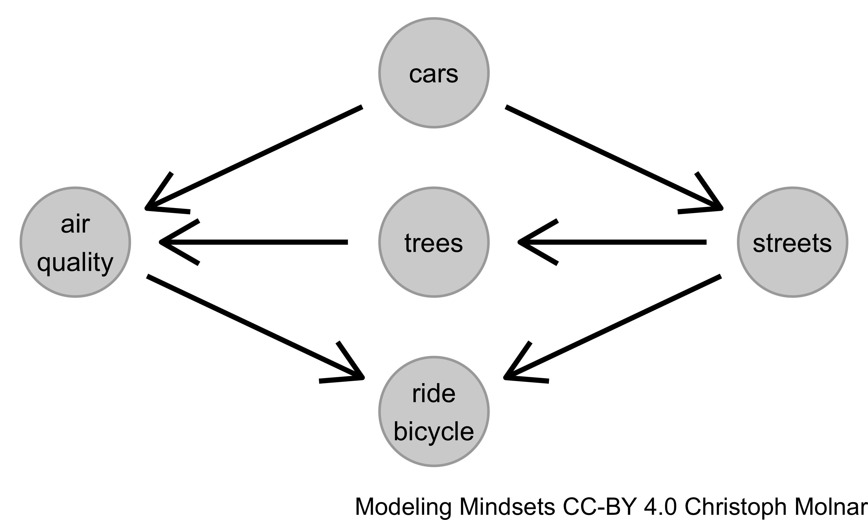
FIGURE 7.2: A directed acyclic graph (DAG) with 5 variables.
What assumptions are made in the DAG in Figure 7.2? Number of cars and number of trees affect air quality (direct causes). The number of streets indirectly affects the air quality through the number of trees (that had to be cut). The number of people that ride bicycle depends on air quality and the number of streets. If the modeler wants to estimate the causal effect of number of streets on air quality, then each variable takes on a different role: cars is a confounder, trees a mediator, and bicycle a collider. Each role comes with different implications for how to deal with them. You might, for example, disagree with the DAG above. Why is there no arrow from cars to bicycle? By making the structures explicit, it’s possible for causal modelers to challenge assumptions.
How does the modeler know how to place the arrows? There are several guides here:
- Good old common sense, such as knowing that park visitors can’t control the sun.
- Domain expertise.
- Direction of time: We know that the elevator comes because you pressed the button, not the other way around.
- Causal structure learning: To some extent we can learn causal structures automatically. But this usually leads to multiple, ambiguous DAGs.
- …
7.4 Many Frameworks For Causality
There are many “schools”, frameworks, and individual models for causal inference. They can differ in notation and approaches. (Hernán and Robins 2010) I find this lack of uniformity one of the biggest barrier to entry into the causal inference mindset. You can choose different introductory books on Bayesian inference, and the basic notation, language and presented methods will mostly be the same. But for causal inference it is a bit more messy. So don’t despair, it’s not your fault. Anyway, here is a brief, far-from-exhaustive overview of causal modeling approaches:
- Much causal inference consists of experimental design rather than causal modeling of observational data, such as clinical trials or A/B tests. Causality claims are derived from randomization and intervention.
- Observational data can resemble an experiment, which some call a “natural experiment”. When John Snow studied cholera, he had access to data from a natural experiment. John Snow identified contaminated drinking water as the source of cholera because customers of one water company were much more likely to get cholera than customers of the other.
- Propensity score matching attempts to estimate the effect of an intervention by matching individuals that are (mostly) identical on a set of background variables.
- Probably the most general and coherent framework for causal inference comes from statistician Judea Pearl. This “school” covers the do-calculus(Pearl 2012), structural causal models, front- and backdoor criteria, and many other tools for causal inference. (Pearl 2009)
- The potential outcomes framework (Holland 1986) is another larger causal “school” used mainly for studying causal effects of binary variables.
- Causal discovery or structure identification is a subfield of causal inference that aims to construct DAGs (in parts) from observational data.
- Mediation analysis can be used to examine how causal effects are mediated by other variables.
- There are many individual methods that aim to provide causal modeling. One example is “honest causal forests”, which are based on random forests and used to model heterogeneity in treatment effects.(Athey and Imbens 2016)
- …
All approaches have in common that they start from a causal model. This causal model can be very explicit, for example in the form of a DAG. But it can also be hidden in the assumptions of a method. The final estimate, however, is always something like a statistical estimator or machine learning model. But how do you get from a causal model to a statistical estimator?
7.5 From Causal Model to Statistical Estimator
In many cases a modeler can’t perform experiments or trials because they are infeasible, too expensive or too time-consuming. But often there is observational data available from which the modeler can try to infer causal effects. However, with observational data, the first casualty is causality – at least from the point of view of non-causalists. But when causal modelers see observational data, they start stretching and warming up their wrists in anticipation of all the DAG-drawing and modeling to come.
Causal modelers say that you can estimate causal effects even for observational data. I am willing to reveal their secret: Causal modelers use high-energy particle accelerators to create black holes. Each black hole contains a parallel universe in which they can study a different what-if scenarios. Joke aside, there is no magic ingredient for estimating causal effects. Causal modeling is mainly a recipe for translating causal models into statistical estimators, in the following 4 steps:(Pearl 2009)
- Formulate causal estimand.
- Construct causal model.
- Identify statistical model.
- Estimate effect.
The first step is to formulate the causal estimand. That means defining the causes and target that we are interested in. The estimand can be the effect of a treatment on a disease outcome. It can be the causal influence of supermarket layout on shopping behavior. Or it can be the extent to which climate change affected a certain heat wave.
Once the causal estimand is formulated, the modeler derives a causal model. The causal model can be in the form of DAG and should include all other variables that are to both cause and target.
In the identification step, the modeler translates the causal model into a statistical estimator. Not all causal estimands can be estimated with observational data. In particular, if a confounder is missing, the causal effect can’t be estimated. Identification can be complicated, but there are at least some simple rules that give first hints for which variables to include and which to exclude:
- Include all confounders, the common causes of both the variable of interest and the outcome. For example in Figure 7.3 the number of cars confounds the relation between number of streets and air quality.
- Exclude colliders. Number of bicycles riders is a collider. Adding colliders to a model opens an unwanted dependence between the cause of study and the target.
- Exclude mediators. Number of trees mediates the effect of streets on air quality. Inclusion in the model depends on the goal of the analysis (direct, indirect, or total effect of streets).
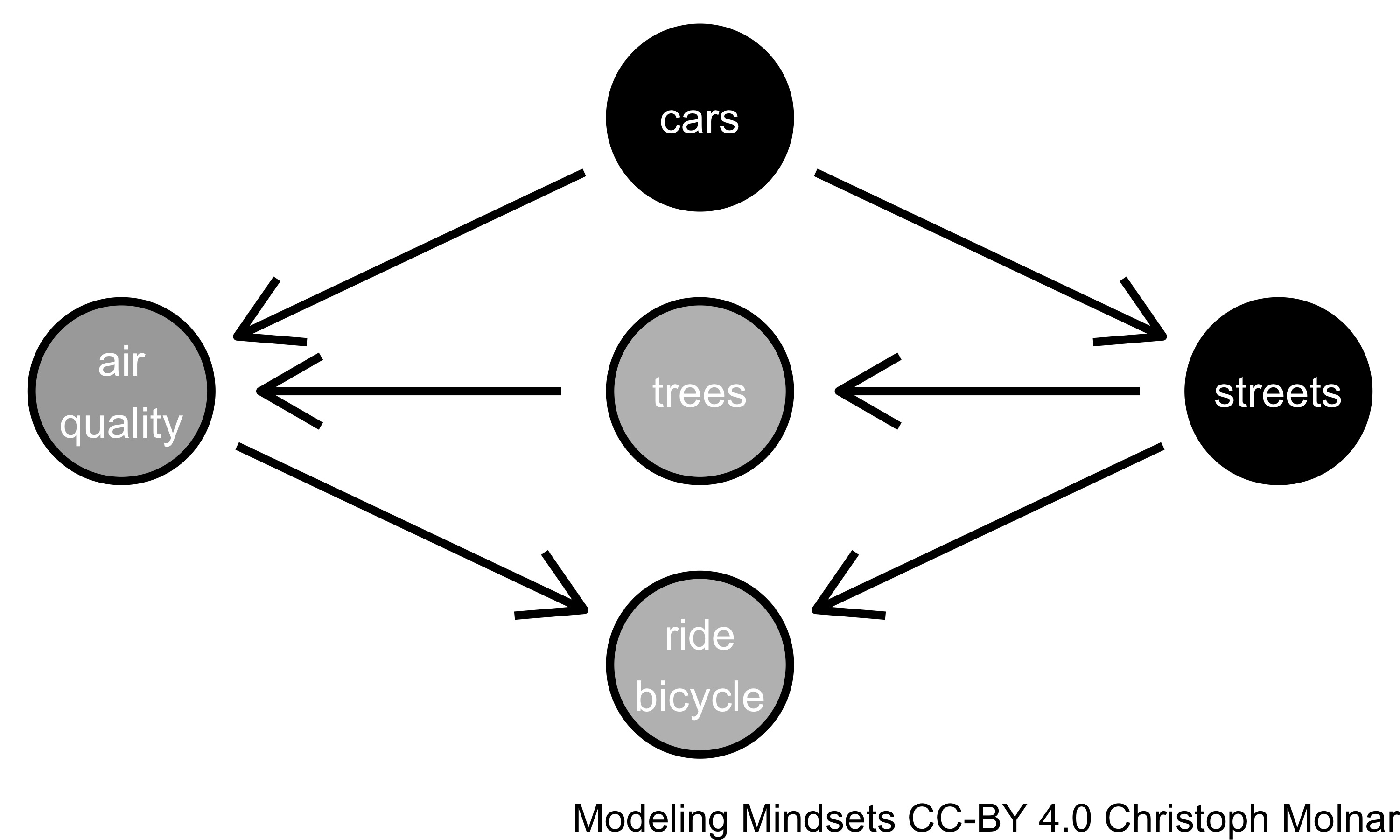
FIGURE 7.3: To understand the (total) causal effect of streets on air quality, a regression model with air quality as the target should include cars and streets as predictor variables.
The result is an estimator that can be fitted with data. The model can be frequentist or Bayesian, but also a supervised machine learning model. To estimate causal effects of other variables, all steps must be repeated. The reason for this is that the identification may lead to a different set of variables for which the model must be adjusted.
7.6 Strengths
- Causality is central to modeling the world.
- Many modelers want their models to be causal. Scientists study causal relationships, data scientists want to understand the impact of, for example, marketing interventions, etc.
- Causal models can be more robust, or put another way: Non-causal models break down more easily, since they are based on associations.
- Causal inference is a rather flexible mindset that extends many other mindsets such as frequentism, Bayesianism, machine learning.
- DAGs make causal assumptions explicit. If you there would be only one takeaway from this chapter, it should be DAGs as a way of thinking and communicating.
7.7 Limitations
- Many modelers stay away from causal inference for observational data because they say causal models are either not possible or too complicated.
- Confounders are tricky. For a causal interpretation, you have to assume that you have found all the confounders. But one can never prove that one has identified all confounders.
- There are many schools and approaches to causal inference. This can be very confusing for newcomers.
- Causal modeling requires subjective decisions. The causal modeler can never be sure that the causal model is correct.
- Predictive performance and causality can be in conflict: Using non-causal variables may improve predictive performance, but may undermine the causal interpretation of the model.
References
Shouldn’t inflammation levels be a confounder because it affects both the decision to treat and the ossification? Or is it a mediator? It depends on the time of the measurement. In the faulty model inflammation was considered after treatment started, making it a mediator of the drug. Later, we adjusted the model to include inflammation before the start of treatment, making it a confounder.↩︎