Chapter 4 Frequentist Inference – Infer Data Generating Process
- Infer fixed but unknown distribution parameters from a data sample
- Estimators of distribution parameters are seen as random variables
- Probability is interpreted as long-run relative frequency
- Hypothesis tests and confidence intervals enable a decision-making mindset
- A statistical mindset, with Bayesian inference and likelihoodism as alternatives.
Once upon a time there was a statistician who dealt p-values. He was the best in the business, and people would flock to him from all over to get their hands on his wares. One day, a young scientist came to the statistician’s shop. The scientist said: “I’m looking for the p-value that will allow me to get my paper published.” The statistician smiled, and reached under the counter. He pulled out a dusty old book, and thumbed through the pages until he found what he was looking for. “The p-value you’re looking for is 0.05,” he said. The scientist’s eyes lit up. “That’s exactly what I need! How much will it cost me?” The statistician leaned in close. “It’ll cost you your soul,” he whispered.
Drinking alcohol is associated with a higher risk of diabetes in middle-aged men. At least this is what a study claims (Kao et al. 2001). The researchers modeled type II diabetes as a function of risk factors. They found that alcohol increased the risk of diabetes by a factor of \(1.81\) for middle-aged men. The researchers used frequentist inference to draw this conclusion from the data. There is no particular reason why I chose this study other than it is a typical study. Modelers that think in significance levels, p-values, hypothesis tests, and confidence intervals are frequentists.
In many scientific fields, such as medicine and psychology, frequentist inference is the dominant modeling mindset. Frequentist papers follow similar patterns, make similar assumptions, and contain similar tables and figures. Understanding frequentist concepts such as confidence intervals and hypothesis tests is therefore one of the keys to understanding scientific progress. Frequentism but has a firm foothold in industry as well: Statisticians, data scientists, and whatever the future name the role will have, often use frequentist inference to create value for businesses, from analyzing A/B tests for a website to calculating portfolio risk to monitoring quality on production lines.
4.1 Frequentism Allows Making Decisions
Frequentist inference is a statistical modeling mindset: It has variables, distributions, and models. Frequentism comes with a specific interpretation of probability: Probability is seen as the relative frequency of an event in infinitely repeated trials. That’s why it’s called frequentism: frequentist inference emphasizes the (relative) frequency of events. But how do these long-run frequencies help to gain insights from the model?
Let’s go back to the \(1.81\) increase in diabetes risk among men who drink a lot of alcohol. \(1.81\) is larger than \(1\), so there seems to be a difference between men who drink alcohol and the ones who don’t. But how can the researchers be sure that the \(1.81\) is not a random result? If you flip a coin 100 times, and it comes up with tails 51 times, our gut-feeling would say that the coin is fair. Probability as long-run frequencies allows to formulate cut-off values within which we would say that the coin is fair, like 40 to 60. Beyond that we would say that the coin is not fair.
The researchers applied the same type of frequentist thinking to decide whether the effect of alcohol is random or not. In the case of the study, the parameter of interest was a coefficient in a logistic regression model. The diabetes study reported a 95% confidence interval for the alcohol coefficient ranging from \(1.14\) to \(2.92\). The interval doesn’t contain \(1\), so the researchers concluded that alcohol is a risk factor for diabetes (in men), or at least significantly associated.
4.2 Frequentism Needs Imagined Experiments
The interpretation of confidence intervals is in the spirit of long-term frequencies: If the statisticians would repeat the analysis many times with new samples, the respective 95% confidence interval would cover the “true” parameter 95% of the time. Always under the condition that the model assumptions were correct. The interpretation of the confidence interval reveals the core philosophy of frequentism:
- Study population parameters through a data sample.
- These parameters are constant and unknown.
- Repeated measurements/experiments reveal the true parameter values in the long-run.
- The parameter estimators are random variables
- Uncertainty is expressed through the variance of these parameter estimators.
As the frequentist collect more and more data, the parameter estimates get closer and closer to the true parameters (if the estimators are unbiased). More data means narrower confidence intervals. With each additional data point, the uncertainty of the estimated parameter shrinks and the confidence interval becomes narrower. In contrast, Bayesianism assumes that the parameters of the distributions are themselves random variables.
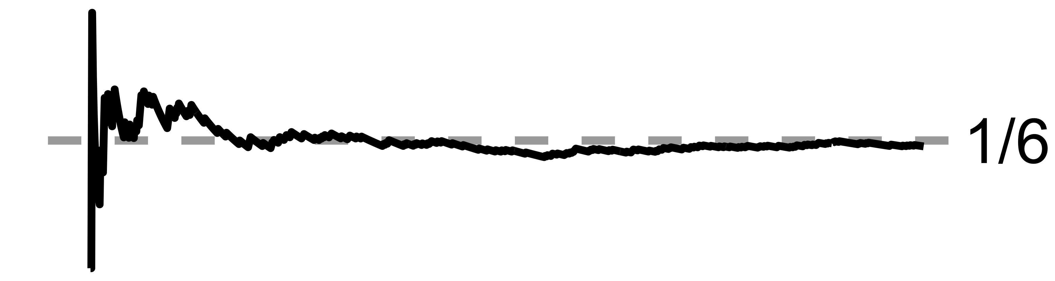
FIGURE 4.1: The line shows how the relative frequency of 6 eyes changes as the number of dice roles increases from 1 to 1000 (left to right).
There is an aspect of confidence intervals that shows what’s special about frequentist inference: it’s interpretation involves imagined experiments. By defining probability in terms of long-run frequencies, frequentism requires imagining that the sampling and experiment will be done many times. Statisticians don’t actually have run these additional experiments. Except when frequentist statisticians propose new estimators for confidence intervals: to prove that the coverage of the interval is correct (it really covers parameter e.g. 95% of the time), simulated experiments are run thousands of times. Imagined experiments are central to the interpretation of confidence intervals, p-values, and hypothesis tests.
4.3 Estimators are Random Variables
It’s going to get a little abstract. The best way to understand frequentism is to work your way slowly from data to estimators to repeated experiments and finally to a decision.
1) Data are random variables
Assume a statistician has observed independent draws of 10 data points for a variable. For the sake of imagination, let’s say the statistician weighs apples and has measured 10 different apples. The variable is: weight of a certain type of apple, and the statistician has 10 observations of this variable. The statistician assumes that the weight variable follows a Gaussian distribution. The statistician wants to know: 1.) What’s the average weight of an apple (including estimates of uncertainty)? And 2.) Does the average apple weigh less than 100g?
2) Estimators are random variables
To answer the question, the statistician first estimates a property of the weight distribution. In this case, the mean of the apples’ weight distribution. The estimation is simple: add all observed values and divide by 10. Let’s say the result is 79. As a function of a random variable, this mean estimator is a random variable itself. And the 79 that the statistician calculated is 1 observation of that random variable.
The mean is one of the simplest estimators. There are many more including more complex ones:
- Coefficients in a logistic regression model
- Estimator of the variance of a random variable
- Correlation coefficient
3) Repeated imaginary experiments
Back to the apples: 79 is smaller than 90. But since the estimator is a random variable, it comes with uncertainty. Assuming that the true average weight is 90, couldn’t a sample of 10 apples weight 79 grams on average, just by chance?
Bad news: The statistician has only 1 observation of the mean estimate and no motivation to buy more apples. Who on earth should eat all those apples? Good news: The statistician can derive the distribution of the mean estimate from the data distribution. Since the apple weights follows a Gaussian distribution, the statistician concludes that the mean estimator follows a Student distribution. This distribution of estimator has to be interpreted in terms of long-run frequency: It tells the statistician what to expect of the mean estimates in future experiments. Of course, given that the supermarket doesn’t change the type of apple. Now the statistician has: An estimate of the average weight of the apple, and even knows the distribution. Enough to quantify the uncertainty of the analysis. The statistician could visualize the distribution of the mean estimate which shows how uncertain the estimate is (helping with question 1). From this visualization the statistician might also eye-ball whether 90 gram seems like a likely outcome. But that’s not good enough for the frequentist.
4) Make a decision
To draw conclusions about the population, the frequentist elaborates how the mean estimate would behave if the experiment were repeated. The experiment was: Sample 10 apples, weigh them, and calculate the average weight. The frequentist has two tools available to make probabilistic statements about the average weight of the apples. One tool is hypothesis tests, the other is confidence intervals. Bold tools that make clear, binary statements about which values are likely and which are not. Through this binary choice, they can be used to make decisions.
4.3.1 Hypothesis tests
A hypothesis test is a method to decide whether the data support a hypothesis. In the apple case: Does the observed average of 79 grams still support the hypothesis of 90 grams average apple weight? 90 grams is also called the null hypothesis. Based on the assumed distributions, the corresponding test would be a one-sample Student t-test. The t-test calculates a p-value which measures how a result of 79 (or extremer) is given that 90 grams is the true average apple weight. If the p-value is below a certain confidence level, then 79 is so far away from 90 that the statisticians reject the 90-hypothesis. Most of the time a confidence level of 5% is chosen. The confidence value means that, if the null hypothesis is really true, the test would falsely reject the hypothesis in 5% of the cases (1 out of 20). This so-called null hypothesis significance testing 4 is popular but also criticized for many reasons.
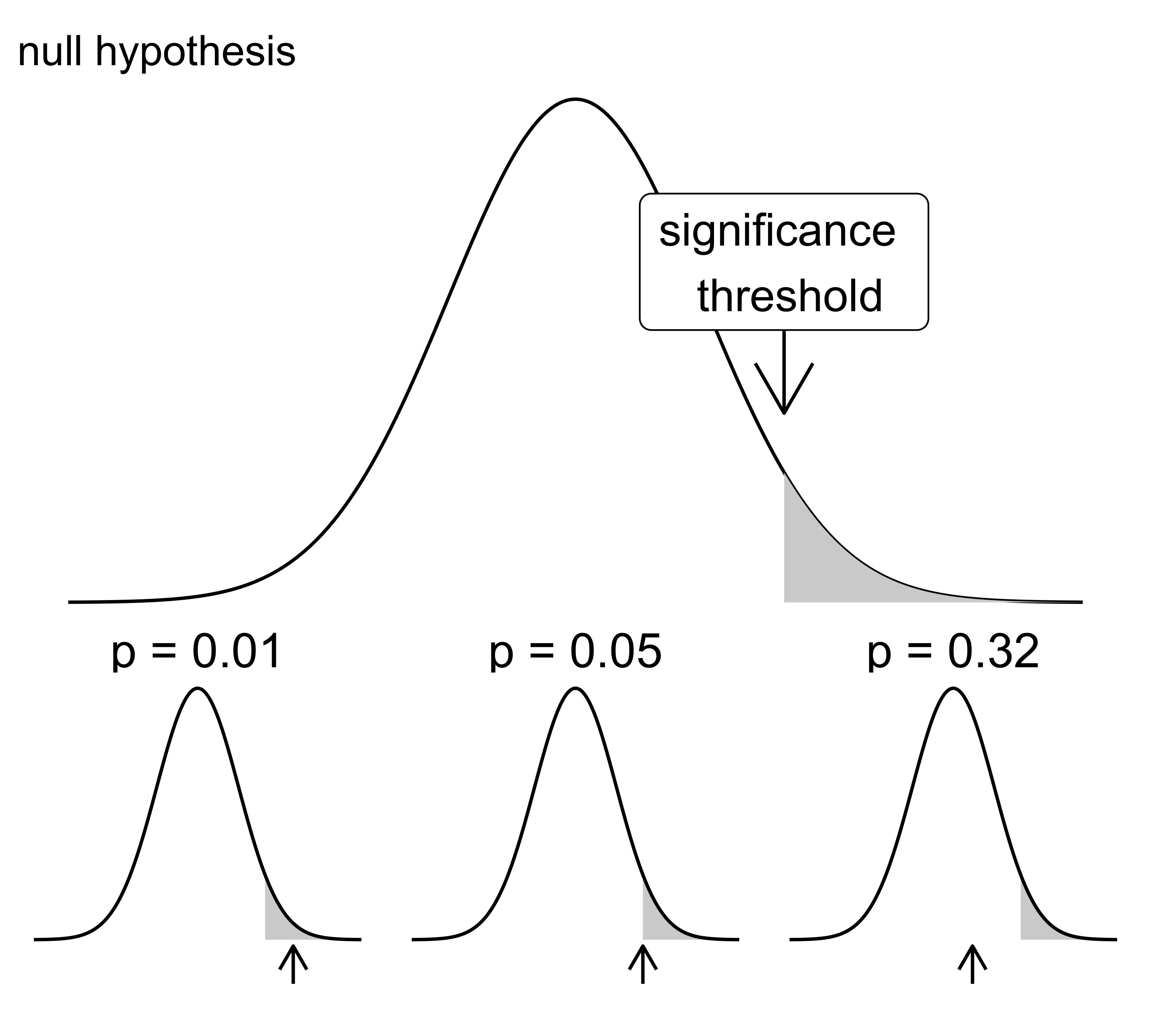
FIGURE 4.2: Frequentists can make binary decisions based on hypothesis tests. If the observed test statistic is too extreme under the (assumed) distribution of the null hypothesis, the null hypothesis is rejected.
4.3.2 Confidence Intervals
Hypothesis tests are criticized for reducing all the information to a yes or no question. Confidence intervals are a more informative alternative. Hypothesis tests and confidence intervals ultimately lead to the same decisions, but confidence intervals are more informative. These intervals that are constructed around the estimate quantify how certain the estimate was: the narrower the more certain. Remember, in the frequentist mindset, it’s about identifying the true parameter which is fixed and unknown. The confidence interval is the region that likely covers the true parameter. But it would be wrong to say: There is 95% chance that the true parameter falls into this interval. A big No-No. If the modeler wants this type of interpretation, better knock on the Bayesians door. But for the frequentist, the experiment is done. Either the parameter is in the resulting interval or it isn’t. Instead the frequentist interprets the 95% confidence interval in terms of long-run frequencies: If the experiment were repeated many times, in 95% of the times the corresponding confidence interval would cover the true parameter. If the statistician were to repeat the experiment 100 times, on average, 95 out of 100 of the resulting confidence intervals would cover the true parameter. A repetition of the experiment means: Draw 10 new apples and compute confidence intervals from this new sample. This sounds like nitpicking … but if you get this distinction, you will have an easy time understanding Bayesian inference.
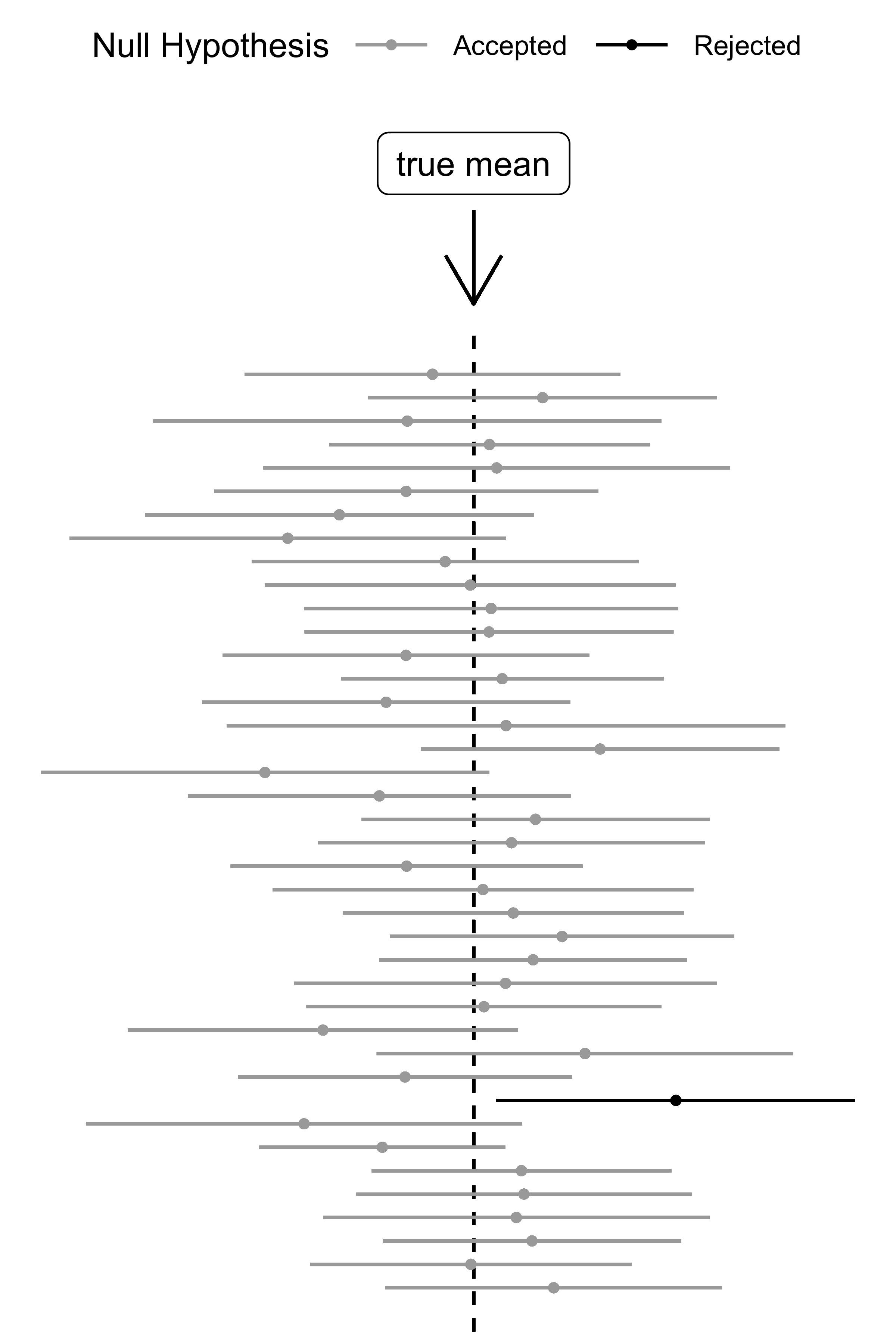
FIGURE 4.3: 20 95% confidence intervals and the true value.
4.4 Strengths
- If you need clear cut answers, frequentist inference it is. This simplicity is one of the reasons why frequentism is popular for both scientific publications and business decisions.
- Once you understand frequentist inference, you can understand the analysis of many research articles.
- Frequentist methods are fast to compute. As a rule-of-thumb faster than methods from Bayesian inference or machine learning.
- Compared to Bayesianism, no prior information about the parameters is required.
- Frequentism has all advantages of statistical models in general: a solid theoretical foundation and an appreciation of the data-generating process.
- When the underlying process is a long-run, repeated experiment, frequentist inference shines. Casino games, model benchmarks, …
4.5 Limitations
- Frequentism incentivizes modelers to over-simplify questions into yes-or-no questions.
- The focus on p-values encourages p-hacking: the search for significant results to get a scientific paper published. P-hacking leads to many false findings in research.
- The frequentist interpretation of probability can be awkward. Especially for confidence intervals. Bayesian credibility intervals seem to have a more “natural” interpretation of uncertainty.
- Frequentist analysis depends not only on the data, but also on the experimental design. This is a violation of the likelihood principle. See the Likelihoodism chapter.
- There is an “off-the-shelf”-mentality among users of frequentist inference. Instead of carefully adapting a probability model to the data, an off-the-shelf hypothesis test or statistical model is chosen.
References
There are two “main” approaches for hypothesis testing: The Fisher approach, and the Neyman-Pearson approach. Null hypothesis significance testing is a combination of the two. (Perezgonzalez 2015)↩︎