22 Functional Decomposition
A supervised machine learning model can be viewed as a function that takes a high-dimensional feature vector as input and produces a prediction or classification score as output. Functional decomposition is an interpretation technique that deconstructs the high-dimensional function and expresses it as a sum of individual feature effects and interaction effects that can be visualized. In addition, functional decomposition is a fundamental principle underlying many interpretation techniques – it helps you better understand other interpretation methods.
Let’s jump right in and look at a particular function. This function takes two features as input and produces a one-dimensional output:
\[\hat{f}(x_1, x_2) = 2 + e^{x_1} - x_2 + x_1 \cdot x_2\]
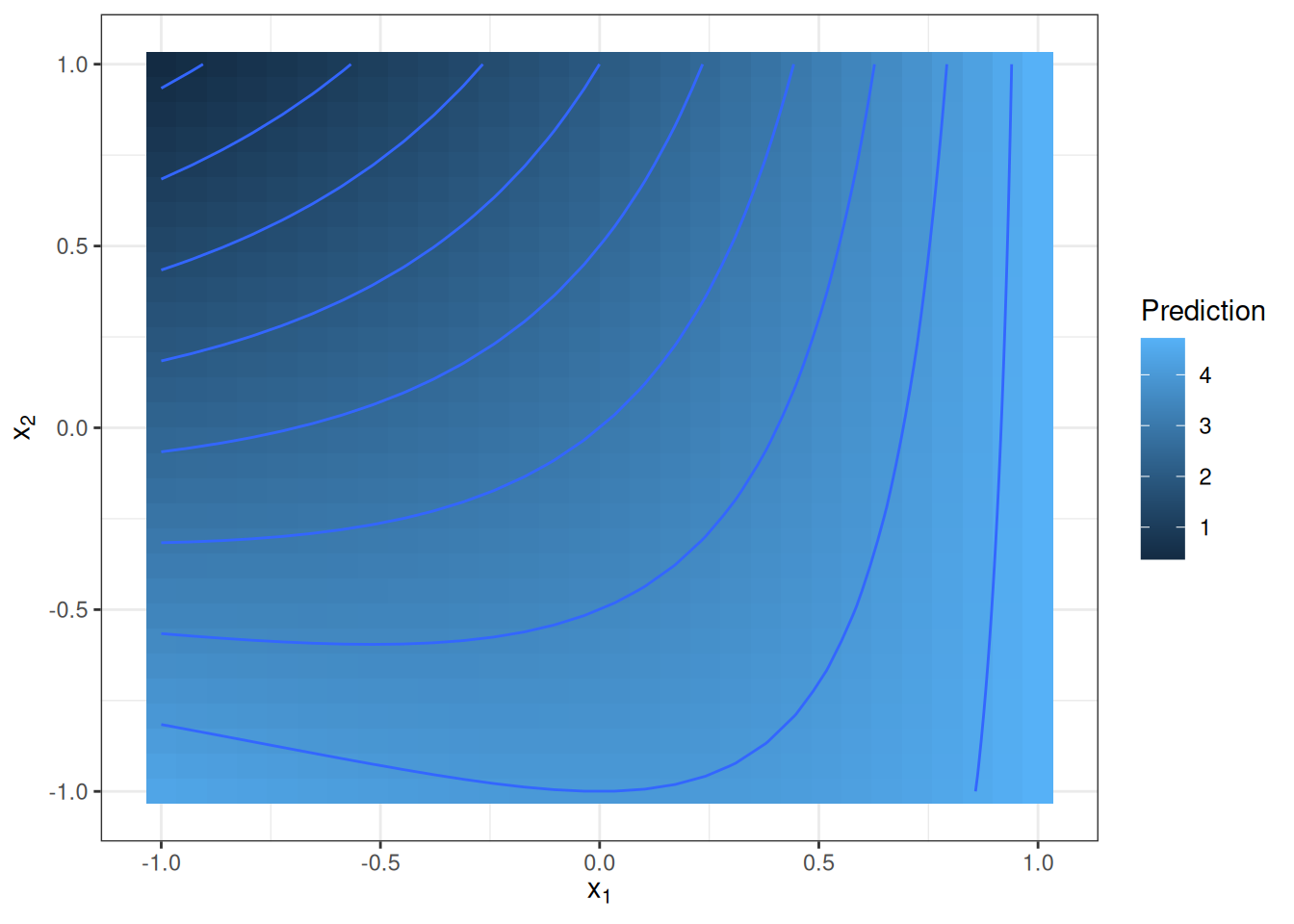
Think of the function as a machine learning model. We can visualize the function with a 3D plot or a heatmap with contour lines as in Figure 22.1.
The function takes large values when \(x_1\) is large and \(x_2\) is small, and it takes small values for large \(x_2\) and small \(x_1\). The prediction function is not simply an additive effect between the two features, but an interaction between the two. The presence of an interaction can be seen in the figure – the effect of changing values for feature \(x_1\) depends on the value that feature \(x_2\) has.
Our job now is to decompose this function into main effects of features \(X_1\) and \(X_2\) and an interaction term. For a two-dimensional function \(\hat{f}\) that depends on only two input features: \(\hat{f}(x_1, x_2)\), we want each component to represent a main effect (\(\hat{f}_1\) and \(\hat{f}_2\)), interaction (\(\hat{f}_{1,2}\)), or intercept (\(\hat{f}_0\)):
\[\hat{f}(x_1, x_2) = \hat{f}_0 + \hat{f}_1(x_1) + \hat{f}_2(x_2) + \hat{f}_{1,2}(x_{1},x_{2})\]
The main effects indicate how each feature affects the prediction, independent of the values the other feature. The interaction effect indicates the joint effect of the features. The intercept is a fixed value that is part of all predictions. If all feature values were set to zero, the prediction would only consist of the intercept. Note that the components themselves are functions (except for the intercept) with different input dimensionality.
I’ll just give you the components now and explain where they come from later. The intercept is given as \(\hat{f}_0 \approx 3.18\). Since the other components are functions, we can visualize them in Figure 22.2.
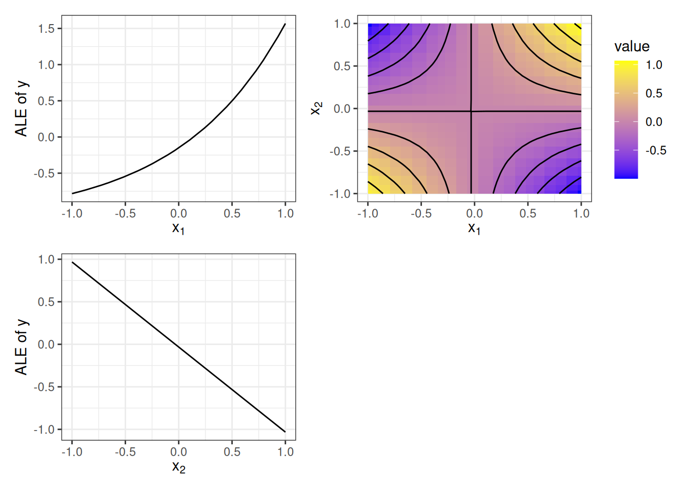
Do you think the components make sense given the above true formula, ignoring that the intercept value seems a bit random? The \(X_1\) feature shows an exponential main effect, and \(X_2\) shows a negative linear effect. The interaction term looks a bit like a Pringles chip. In less crunchy and more mathematical terms, it’s a hyperbolic paraboloid, as we would expect for \(x_1 \cdot x_2\). Spoiler alert: the decomposition is based on accumulated local effect plots, which we will discuss later in the chapter.
But why all the excitement? A glance at the formula already gives us the answer to the decomposition, so no need for fancy methods, right? For feature \(X_1\), we can take all the summands that contain only \(x_1\) as the component for that feature. That would be \(\hat{f}_1(x_1) = e^{x_1}\) and \(\hat{f}_2(x_2) = -x_2\) for feature \(X_2\). The interaction is then \(\hat{f}_{12}(x_{1},x_{2}) = x_1 \cdot x_2\). While this is the correct answer for this example (up to constants), there are two problems with this approach: Problem 1): While the example started with the formula, the reality is that only structurally simple machine learning models can be described with such a neat formula. Problem 2) is much more intricate and concerns what an interaction is. Imagine a simple function \(\hat{f}(x_1,x_2) = x_1 \cdot x_2\), where both features take values larger than zero and are independent of each other. Using our look-at-the-formula tactic, we would conclude that there is an interaction between features \(X_1\) and \(X_2\), but not individual feature effects. But can we really say that feature \(x_1\) has no individual effect on the prediction function? Regardless of what value \(x_2\) takes on, the prediction increases as we increase \(x_1\). For example, for \(x_2 = 1\), the effect of \(x_1\) is \(\hat{f}(x_1, 1) = x_1\), and when \(x_2 = 10\) the effect is \(\hat{f}(x_1, 10) = 10 \cdot x_1\). Thus, it’s clear that feature \(X_1\) has a positive effect on the prediction, independent of \(X_2\), and is not zero.
To solve problem 1) of lack of access to a neat formula, we need a method that uses only the prediction function or classification score. To solve problem 2) of lack of definition, we need some axioms that tell us what the components should look like and how they relate to each other. But first, we should define more precisely what functional decomposition is.
Decomposing a function
A prediction function takes \(p\) features as input, \(\hat{f}: \mathbb{R}^p \mapsto \mathbb{R}\), and produces an output. This can be a regression function, but it can also be the classification probability for a given class or the score for a given cluster (unsupervised machine learning). Fully decomposed, we can represent the prediction function as the sum of functional components:
\[\begin{align*} \hat{f}(\mathbf{x}) = & \hat{f}_0 + \hat{f}_1(x_1) + \ldots + \hat{f}_p(x_p) \\ & + \hat{f}_{1,2}(x_1, x_2) + \ldots + \hat{f}_{1,p}(x_1, x_p) + \ldots + \hat{f}_{p-1,p}(x_{p-1}, x_p) \\ & + \ldots \\ & + \hat{f}_{1,\ldots,p}(x_1, \ldots, x_p) \end{align*}\]
We can make the decomposition formula a bit nicer by indexing all possible subsets of feature combinations: \(S\subseteq\{1,\ldots,p\}\). This set contains the intercept (\(S=\emptyset\)), main effects (\(|S|=1\)), and all interactions (\(|S|\geq{}1\)). With this subset defined, we can write the decomposition as follows:
\[\hat{f}(\mathbf{x}) = \sum_{S\subseteq\{1,\ldots,p\}} \hat{f}_S(\mathbf{x}_S)\]
In the formula, \(\mathbf{x}_S\) is the vector of features in the index set \(S\). And each subset \(S\) represents a functional component, for example, a main effect if \(S\) contains only one feature, or an interaction if \(|S| > 1\).
How many components are in the above formula? The answer boils down to how many possible subsets \(S\) of the features \(1,\ldots, p\) we can form. And these are \(\sum_{i=0}^p\binom{p}{i}=2^p\) possible subsets! For example, if a function uses 10 features, we can decompose the function into 1,024 components: 1 intercept, 10 main effects, 90 2-way interaction terms, 720 3-way interaction terms, … And with each additional feature, the number of components doubles. Clearly, for most functions, it is not feasible to compute all components. Another reason NOT to compute all components is that components with \(|S|>2\) are difficult to visualize and interpret.
So far I’ve avoided talking about how the components are defined and computed. The only constraints we have implicitly talked about were the number and dimensionality of the components, and that the sum of components should yield the original function. But without further constraints on what the components should be, they are not unique. This means we could shift effects between main effects and interactions, or lower-order interactions (few features) and higher-order interactions (more features). In the example at the beginning of the chapter, we could set both main effects to zero and add their effects to the interaction effect.
Here’s an even more extreme example that illustrates the need for constraints on components. Suppose you have a 3-dimensional function. It does not really matter what this function looks like, but the following decomposition would always work: \(\hat{f}_0\) is 0.12. \(\hat{f}_1(\mathbf{x})=2\cdot{}x_1 + \text{number of shoes you own}\). \(\hat{f}_2\), \(\hat{f}_3\), \(\hat{f}_{1,2}\), \(\hat{f}_{2,3}\), \(\hat{f}_{1,3}\) are all zero. And to make this trick work, I define \(\hat{f}_{1,2,3}(x_1,x_2,x_3)=\hat{f}(\mathbf{x})-\sum\limits_{S\subset\{1,\ldots,p\}}\hat{f}_S(\mathbf{x}_S)\). So the interaction term containing all features simply sucks up all the remaining effects, which by definition always works, in the sense that the sum of all components gives us the original prediction function. This decomposition would not be very meaningful and quite misleading if you were to present this as the interpretation of your model.
The ambiguity can be avoided by specifying further constraints or specific methods for computing the components. In this chapter, we will discuss different approaches to functional decomposition:
- (Generalized) functional ANOVA
- Accumulated Local Effects
- Statistical regression models
- Decomposing tree ensembles
Functional ANOVA
Functional ANOVA was proposed by Hooker (2004). A requirement for this approach is that the model prediction function \(\hat{f}\) is square integrable. As with any functional decomposition, the functional ANOVA decomposes the function into components:
\[\hat{f}(\mathbf{x}) = \sum_{S \subseteq \{1, \ldots, p\}} \hat{f}_S(\mathbf{x}_S)\]
Hooker (2004) defines each component with the following formula:
\[\hat{f}_S(\mathbf{x}) = \int_{X_{-S}} \left( \hat{f}(\mathbf{x}) - \sum_{V \subset S} \hat{f}_V(\mathbf{x})\right) d \mathbb{P}(X_{-S})\]
Okay, let’s take this thing apart. We can rewrite the component as:
\[\hat{f}_S(\mathbf{x}) = \int_{X_{-S}} \left( \hat{f}(\mathbf{x})\right) d \mathbb{P}(X_{-S}) - \int_{X_{-S}} \left(\sum_{V \subset S} \hat{f}_V(\mathbf{x}) \right) d \mathbb{P}(X_{-S})\]
On the left side is the integral over the prediction function with respect to the features excluded from the set \(S\), denoted with \(-S\). For example, if we compute the 2-way interaction component for features 2 and 3, we would integrate over features 1, 4, 5, … The integral can also be viewed as the expected value of the prediction function with respect to \(X_{-S}\), assuming that all features follow a uniform distribution from their minimum to their maximum. From this interval, we subtract all components with subsets of \(S\). This subtraction removes the effect of all lower-order effects and centers the effect. For \(S=\{1,2\}\), we subtract the main effects of both features \(\hat{f}_1\) and \(\hat{f}_2\), as well as the intercept \(\hat{f}_0\). The occurrence of these lower-order effects makes the formula recursive: We have to go through the hierarchy of subsets to the intercept and compute all these components. For the intercept component \(\hat{f}_0\), the subset is the empty set \(S=\{\emptyset\}\) and therefore \(-S\) contains all features:
\[\hat{f}_0(\mathbf{x}) = \int_{X} \hat{f}(\mathbf{x}) d \mathbb{P}(X)\]
This is simply the prediction function integrated over all features. The intercept can also be interpreted as the expectation of the prediction function when we assume that all features are uniformly distributed. Now that we know \(\hat{f}_0\), we can compute \(\hat{f}_1\) (and equivalently \(\hat{f}_2\)):
\[\hat{f}_1(\mathbf{x}) = \int_{X_{-1}} \left( \hat{f}(\mathbf{x}) - \hat{f}_0\right) d \mathbb{P}(X_{-1})\]
To finish the calculation for the component \(\hat{f}_{1,2}\), we can put everything together:
\[\begin{align*} \hat{f}_{1,2}(\mathbf{x}) &= \int_{X_{3,4}} \left( \hat{f}(\mathbf{x}) - (\hat{f}_0 + \hat{f}_1(\mathbf{x}) - \hat{f}_0 + \hat{f}_2(\mathbf{x}) - \hat{f}_0)\right) d \mathbb{P}(X_{3},X_4) \\ &= \int_{X_{3,4}} \left(\hat{f}(\mathbf{x}) - \hat{f}_1(\mathbf{x}) - \hat{f}_2(\mathbf{x}) + \hat{f}_0\right) d \mathbb{P}(X_{3},X_4) \end{align*}\]
This example shows how each higher-order effect is defined by integrating over all other features, but also by removing all the lower-order effects that are subsets of the feature set we are interested in.
Hooker (2004) has shown that this definition of functional components satisfies these desirable axioms:
- Zero Means: \(\int \hat{f}_S(\mathbf{x}_S)d \mathbb{P}(X_S)=0\) for each \(S\neq\emptyset\).
- Orthogonality: \(\int \hat{f}_S(\mathbf{x}_S)\hat{f}_V(\mathbf{x}_V)d \mathbb{P}(X)=0\) for \(S\neq V\).
- Variance Decomposition: Let \(\sigma^2_{\hat{f}}=\int \hat{f}(\mathbf{x})^2d \mathbb{P}(X)\), then \(\sigma^2(\hat{f}) = \sum_{S \subseteq P} \sigma^2_S(\hat{f}_S)\), where \(P=\{1,\ldots,p\}\).
The zero means axiom implies that all effects or interactions are centered around zero. As a consequence, the interpretation at a position \(\mathbf{x}\) is relative to the centered prediction and not the absolute prediction.
The orthogonality axiom implies that components do not share information. For example, the first-order effect of feature \(X_1\) and the interaction term of \(X_{1}\) and \(X_2\) are not correlated. Because of orthogonality, all components are “pure” in the sense that they do not mix effects. It makes a lot of sense that the component for, say, feature \(X_4\) should be independent of the interaction term between features \(X_1\) and \(X_2\). The more interesting consequence arises for orthogonality of hierarchical components, where one component contains features of another, for example, the interaction between \(X_1\) and \(X_2\), and the main effect of feature \(X_1\). In contrast, a two-dimensional partial dependence plot for \(X_1\) and \(X_2\) would contain four effects: the intercept, the two main effects of \(X_1\) and \(X_2\), and the interaction between them. The functional ANOVA component for \(\hat{f}_{1,2}(x_1,x_2)\) contains only the pure interaction.
Variance decomposition allows us to divide the variance of the function \(\hat{f}\) among the components and guarantees that it adds up to the total variance of the function in the end. The variance decomposition property can also explain to us why the method is called functional ANOVA. In statistics, ANOVA stands for ANalysis Of VAriance. ANOVA refers to a collection of methods that analyze differences in the mean of a target variable. ANOVA works by dividing the variance and attributing it to the variables. Functional ANOVA can therefore be seen as an extension of this concept to any function.
Problems arise with the functional ANOVA when features are correlated. As a solution, Hooker (2007) proposed the generalized functional ANOVA.
Generalized Functional ANOVA for dependent features
Similar to most interpretation techniques based on sampling data (such as the PDP), the functional ANOVA can produce misleading results when features are correlated. If we integrate over the uniform distribution, when in reality features are dependent, we create a new dataset that deviates from the joint distribution and extrapolates to unlikely combinations of feature values.
Hooker (2007) proposed the generalized functional ANOVA, a decomposition that works for dependent features. It’s a generalization of the functional ANOVA we encountered earlier, which means that the functional ANOVA is a special case of the generalized functional ANOVA. The components are defined as projections of \(\hat{f}\) onto the space of additive functions:
\[\hat{f}_S(\mathbf{x}_S) = \arg\min_{g_S \in L^2(\mathbb{R}^S)_{S \in P}} \int \left(\hat{f}(\mathbf{x}) - \sum_{S \subset P} g_S(\mathbf{x}_S)\right)^2 w(\mathbf{x})\,d\mathbf{x}.\]
Instead of orthogonality, the components satisfy a hierarchical orthogonality condition:
\[\forall \hat{f}_S(\mathbf{x}_S)| S \subset U: \int \hat{f}_S(\mathbf{x}_S) \hat{f}_U(\mathbf{x}_U) w(\mathbf{x})\,d\mathbf{x} = 0\]
Hierarchical orthogonality is different from orthogonality. For two feature sets \(S\) and \(U\), neither of which is a subset of the other (e.g., \(S=\{1,2\}\) and \(U=\{2,3\}\)), the components \(\hat{f}_S\) and \(\hat{f}_U\) need not be orthogonal for the decomposition to be hierarchically orthogonal. But all components for all subsets of \(S\) must be orthogonal to \(\hat{f}_S\). As a result, the interpretation differs in relevant ways: Similar to the M-Plot in the ALE chapter, generalized functional ANOVA components can entangle the (marginal) effects of correlated features. Whether the components entangle the marginal effects also depends on the choice of weight function \(w(\mathbf{x})\). If we choose \(w\) to be the uniform measure on the unit cube, we obtain the functional ANOVA from the section above. A natural choice for \(w\) is the joint probability distribution function. However, the joint distribution is usually unknown and difficult to estimate. A trick can be to start with the uniform measure on the unit cube and cut out areas without data.
The estimation is done on a grid of points in the feature space and is stated as a minimization problem that can be solved using regression techniques. However, the components cannot be computed independently of each other, nor hierarchically, but a complex system of equations involving other components has to be solved. The computation is therefore quite complex and computationally intensive.
Accumulated Local Effects
ALE plots (Apley and Zhu 2020) also provide a functional decomposition, meaning that adding all ALE plots from intercept, 1D ALE plots, 2D ALE plots, and so on yields the prediction function. ALE differs from the (generalized) functional ANOVA, as the components are not orthogonal but, as the authors call it, pseudo-orthogonal. To understand pseudo-orthogonality, we have to define the operator \(H_S\), which takes a function \(\hat{f}\) and maps it to its ALE plot for feature subset \(S\). For example, the operator \(H_{1,2}\) takes as input a machine learning model and produces the 2D ALE plot for features 1 and 2: \(H_{1,2}(\hat{f}) = \hat{f}_{ALE,12}\). If we apply the same operator twice, we get the same ALE plot. After applying the operator \(H_{1,2}\) to \(\hat{f}\) once, we get the 2D ALE plot \(\hat{f}_{ALE,12}\). Then we apply the operator again, not to \(\hat{f}\) but to \(\hat{f}_{ALE,12}\). This is possible because the 2D ALE component is itself a function. The result is again \(\hat{f}_{ALE,12}\), meaning we can apply the same operator several times and always get the same ALE plot. This is the first part of pseudo-orthogonality. But what is the result if we apply two different operators for different feature sets? For example, \(H_{1,2}\) and \(H_{1}\), or \(H_{1,2}\) and \(H_{3,4,5}\)? The answer is zero. If we first apply the ALE operator \(H_S\) to a function and then apply \(H_U\) to the result (with \(S \neq U\)), then the result is zero. In other words, the ALE plot of an ALE plot is zero, unless you apply the same ALE plot twice. Or in other words, the ALE plot for the feature set \(S\) does not contain any other ALE plots in it. Or in mathematical terms, the ALE operator maps functions to orthogonal subspaces of an inner product space.
As Apley and Zhu (2020) note, pseudo-orthogonality may be more desirable than hierarchical orthogonality because it does not entangle marginal effects of the features. Furthermore, ALE does not require estimation of the joint distribution; the components can be estimated in a hierarchical manner, which means that calculating the 2D ALE for features 1 and 2 requires only the calculations of individual ALE components of 1 and 2, and the intercept term in addition.
Does the Partial Dependence Plot also provide a functional decomposition? Short answer: No. Longer answer: The partial dependence plot for a feature set \(S\) always contains all effects of the hierarchy – the PDP for \(\{1,2\}\) contains not only the interaction, but also the individual feature effects. As a consequence, adding all PDPs for all subsets does not yield the original function, and thus is not a valid decomposition. But could we adjust the PDP, perhaps by removing all lower effects? Yes, we could, but we would get something similar to the functional ANOVA. However, instead of integrating over a uniform distribution, the PDP integrates over the marginal distribution of \(X_{-S}\), which is estimated using Monte Carlo sampling.
Decomposing tree ensembles
Yang et al. (2024) proposed a functional decomposition of tree ensembles, for example, trained with XGBoost. Their proposal consists of two parts: a decomposition procedure and a set of training constraints to make the decomposition more interpretable.
The strategy to get from an ensemble of trees to the functional composition involves aggregation, purification, and attribution. First, each tree is decomposed into decision rules, with each leaf node becoming a decision rule. These rules are then sorted by the features they use. For example, all rules using only feature \(X_1\) are collected and used to estimate the main effect \(\hat{f}_1\). The same is done for all other main effects and interactions. However, this decomposition wouldn’t be unique since, for example, you could absorb the main effect of \(X_1\) into the interaction term of \(X_1\) and \(X_2\). They “purify” the components to enforce zero means and orthogonality constraints (should sound familiar by now). In the attribution step, feature contributions for each data point are computed and aggregated across the data to get global importance values for each feature. The individual contributions are the same as the Shapley values.
The other suggestion in the paper is to add constraints to the training so that the functional decomposition can be better interpreted. This includes simple things like setting the maximum tree depth low so that you control the maximum number of features that can interact. For example, setting the maximum depth to two makes the model have only main effects and two-way interactions, but no higher-order interactions. Other suggestions include monotonicity constraints, reduced number of bins, and interaction constraints. They also introduce a post-processing step for pruning effects from the functional decomposition.
Statistical regression models
This approach ties in with interpretable models, in particular generalized additive models. Instead of decomposing a complex function, we can build constraints into the modeling process so that we can easily read out the individual components. While decomposition can be handled in a top-down manner, where we start with a high-dimensional function and decompose it, generalized additive models provide a bottom-up approach, where we build the model from simple components. Both approaches have in common that their goal is to provide individual and interpretable components. In statistical models, we restrict the number of components so that not all \(2^p\) components have to be fitted. The simplest version is linear regression:
\[\hat{f}(\mathbf{x}) = \beta_0 + \beta_1 x_1 + \ldots + \beta_p x_p\]
The formula looks very similar to the functional decomposition, but with two major modifications. Modification 1: All interaction effects are excluded, and we keep only the intercept and main effects. Modification 2: The main effects may only be linear in the features: \(\hat{f}_j(x_j) = \beta_j x_j\). Viewing the linear regression model through the lens of functional decomposition, we see that the model itself represents a functional decomposition of the true function that maps from features to target, but under strong assumptions that the effects are linear effects and there are no interactions.
The generalized additive model relaxes the second assumption by allowing more flexible functions \(\hat{f}_j\) through the use of splines. Interactions can also be added, but this process is rather manual. Approaches such as GA2M attempt to add 2-way interactions automatically to a GAM (Caruana et al. 2015).
Thinking of a linear regression model or a GAM as functional decomposition can also lead to confusion. If you apply the decomposition approaches from earlier in the chapter (generalized functional ANOVA and accumulated local effects), you may get components that are different from the components read directly from the GAM. This can happen when interaction effects of correlated features are modeled in the GAM. The discrepancy occurs because other functional decomposition approaches split effects differently between interactions and main effects.
So when should you use GAMs instead of a complex model + decomposition? You should stick to GAMs when most interactions are zero, especially when there are no interactions with three or more features. If we know that the maximum number of features involved in interactions is two (\(|S| \leq 2\)), then we can use approaches like MARS or GA2M. Ultimately, model performance on test data may indicate whether a GAM is sufficient or a more complex model performs much better.
Strengths
I consider functional decomposition to be a key concept of machine learning interpretability that helps to better understand many other methods.
Functional decomposition gives us a theoretical justification for decomposing high-dimensional and complex machine learning models into individual effects and interactions – a necessary step that allows us to interpret individual effects. Functional decomposition is the core idea for techniques such as statistical regression models, ALE, (generalized) functional ANOVA, PDP, the H-statistic, and ICE curves.
Functional decomposition also provides a better understanding of other methods. For example, permutation feature importance breaks the association between a feature and the target. Viewed through the functional decomposition lens, we can see that the permutation “destroys” the effect of all components in which the feature was involved. This affects the main effect of the feature, but also all interactions with other features. As another example, Shapley values decompose a prediction into additive effects of the individual features. But the functional decomposition tells us that there should also be interaction effects in the decomposition, so where are they? Shapley values provide a fair attribution of effects to the individual features, meaning that all interactions are also fairly attributed to the features and therefore divided up among the Shapley values.
When considering functional decomposition as a tool, the use of ALE plots offers many advantages. ALE plots provide a functional decomposition that is fast to compute, has software implementations (see the ALE chapter), and desirable pseudo-orthogonality properties.
Limitations
The concept of functional decomposition quickly reaches its limits for high-dimensional components beyond interactions between two features. Not only does this exponential explosion in the number of features limit practicability, since we cannot easily visualize higher-order interactions, but computational time is insane if we were to compute all interactions.
Each method of functional decomposition has its individual disadvantages. The bottom-up approach – constructing regression models – is a quite manual process and imposes many constraints on the model that can affect predictive performance. Functional ANOVA requires independent features. Generalized functional ANOVA is very difficult to estimate. Accumulated local effect plots do not provide a variance decomposition.
The functional decomposition approach is more appropriate for analyzing tabular data than text or images.