23 Permutation Feature Importance
Permutation feature importance (PFI) measures the increase in the prediction error of the model after we permute the values of the feature, which breaks the relationship between the feature and the true outcome.
The concept is really straightforward: A feature is “important” if shuffling its values increases the model error, because in this case, the model relied on the feature for the prediction. A feature is “unimportant” if shuffling its values leaves the model error unchanged, because in this case, the model ignored the feature for the prediction.
Theory
The permutation feature importance measurement was introduced by Breiman (2001) for random forests. Based on this idea, Fisher, Rudin, and Dominici (2019) proposed a model-agnostic version of the feature importance and called it model reliance. They also introduced more advanced ideas about feature importance, for example, a (model-specific) version that takes into account that many prediction models may predict the data well. Their paper is worth reading.
The permutation feature importance algorithm based on Fisher, Rudin, and Dominici (2019):
Input: Trained model \(\hat{f}\), feature matrix \(\mathbf{X}\), target vector \(\mathbf{y}\), error measure \(L\).
- Estimate the original model error \(e_{orig} = \frac{1}{n_{test}} \sum_{i=1}^{n_{test}} L(y^{(i)}, \hat{f}(\mathbf{x}^{(i)}))\) (e.g., mean squared error).
- For each feature \(j \in \{1,...,p\}\) do:
- Generate feature matrix \(\mathbf{X}_{perm,j}\) by permuting feature j in the data \(\mathbf{X}\). This breaks the association between feature j and true outcome y.
- Estimate error \(e_{perm,j} = \frac{1}{n_{test}} \sum_{i=1}^{n_{test}} L(y^{(i)},\hat{f}(\mathbf{x}_{perm,j}))\) based on the predictions of the permuted data.
- Calculate permutation feature importance as quotient \(FI_j= e_{perm}/e_{orig}\) or difference \(FI_j = e_{perm,j}- e_{orig}\)
- Sort features by descending FI.
Invert positive metrics
You can also use PFI with metrics where larger is better, like accuracy or AUC. Just make sure to swap the roles of \(e_{\text{perm}}\) and \(e_{\text{orig}}\) in the ratio/difference.
Fisher, Rudin, and Dominici (2018) suggest in their paper to split the dataset in half and swap the values of feature j of the two halves instead of permuting feature j. This is exactly the same as permuting feature j if you think about it. If you want a more accurate estimate, you can estimate the error of permuting feature j by pairing each instance with the value of feature j of each other instance (except with itself). This gives you a dataset of size n(n-1) to estimate the permutation error, and it takes a large amount of computation time. I can only recommend using the n(n-1)-method if you are serious about getting extremely accurate estimates.
Use unseen data for PFI
Estimate PFI on data not used for model training to avoid overly optimistic results, especially with overfitting models. PFI on training data can falsely highlight irrelevant features as important due to model overfitting.
To understand which features the model actually used, consider alternatives like SHAP importance or PDP importance, which don’t rely on error measures.
In the examples, I used test data to compute permutation feature importance.
Example and interpretation
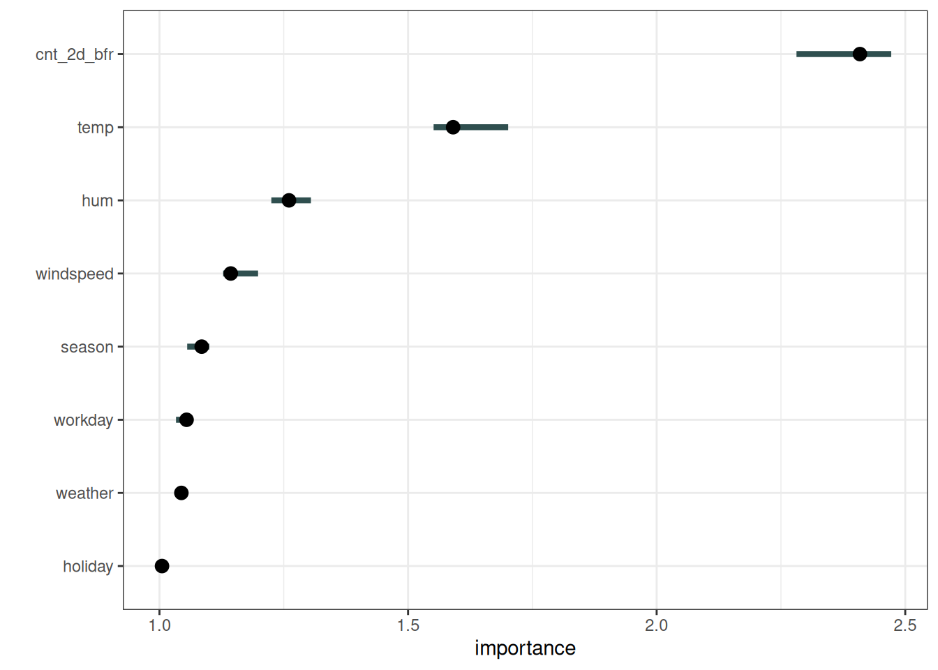
For the first example, we explain the support vector machine model trained to predict the number of rented bikes, given weather conditions and calendar information. As error measurement, we use the mean absolute error. Figure 23.1 shows the permutation feature importance results. The most important feature was cnt_2d_bfr, and the least important was holiday.
Next, let’s look at penguins. I trained 3 logistic regression models to predict penguin sex, using 2/3 of the data for training, and 1/3 for computing the importance. I measure the error as the log loss. Features associated with a model error increase by a factor of 1 (= no change) were not important for predicting penguin male vs. female, as Figure 23.2 shows.
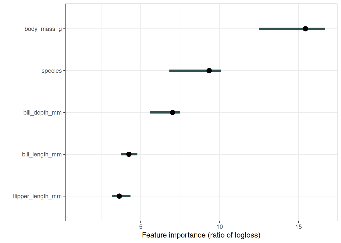
The importance of each of the features for predicting penguin sex with the logistic regression models. The most important feature was body_mass_g. Permuting body_mass_g resulted in an increase in classification error by a factor of 15.4. But wait, how can species be an important feature as well, when I actually trained 3 models separately? I treated the 3 models as one black box model here. To this overall function, species appears as just another feature. Internally this feature splits the data, dispatches it to the three logistic regression models.
Conditional feature importance
Like all the model-agnostic methods, permutation feature importance has a problem when features are dependent. Shuffling produces unrealistic or at least unlikely data points, that are then used to compute feature importance – not ideal. The problem is the marginal version of PFI ignores dependencies. But there is also the concept of conditional importance. The conditional version samples from the conditional distribution \(\mathbb{P}(X_j | X_{-j})\) instead of the marginal distribution \(\mathbb{P}(X_j)\) (shuffling is a way to sample from the marginal distribution). By conditional sampling, we sample more realistic data points.
However, sampling from the conditional distribution is difficult. It’s an even more difficult task than our original machine learning task. But it can be simplified by making assumptions such as assuming a feature is only linearly correlated with other features. Here are some options for conditional sampling:
- Compute PFI in subgroups of the data and aggregate them. Subgroups are based on splitting in correlated features (Molnar et al. 2023).
- Use matching and imputation techniques to generate samples from the conditional distribution (Fisher, Rudin, and Dominici 2019).
- Use knockoffs (Watson and Wright 2021).
- For random forests, there is a model-specific implementation Debeer and Strobl (2020), based on the original random forest importance (Breiman 2001).
Conditional feature importance has a different interpretation from marginal PFI:
- PFI measures the loss increase due to losing the feature information.
- Conditional importance measures the loss increase due to losing the information unique to that feature, information not encoded in other features.
Conditional importance can be a bit more difficult to interpret, since you also need an understanding of how features are dependent on each other. That’s why I’m a big fan of the subgroups approach (and wrote a paper about it): Computing the PFI by group allows you to keep the marginal interpretation.
Correlated features have lower conditional importance
Strongly dependent features usually have very low conditional importance, even when they are used by the model.
Group-wise PFI example
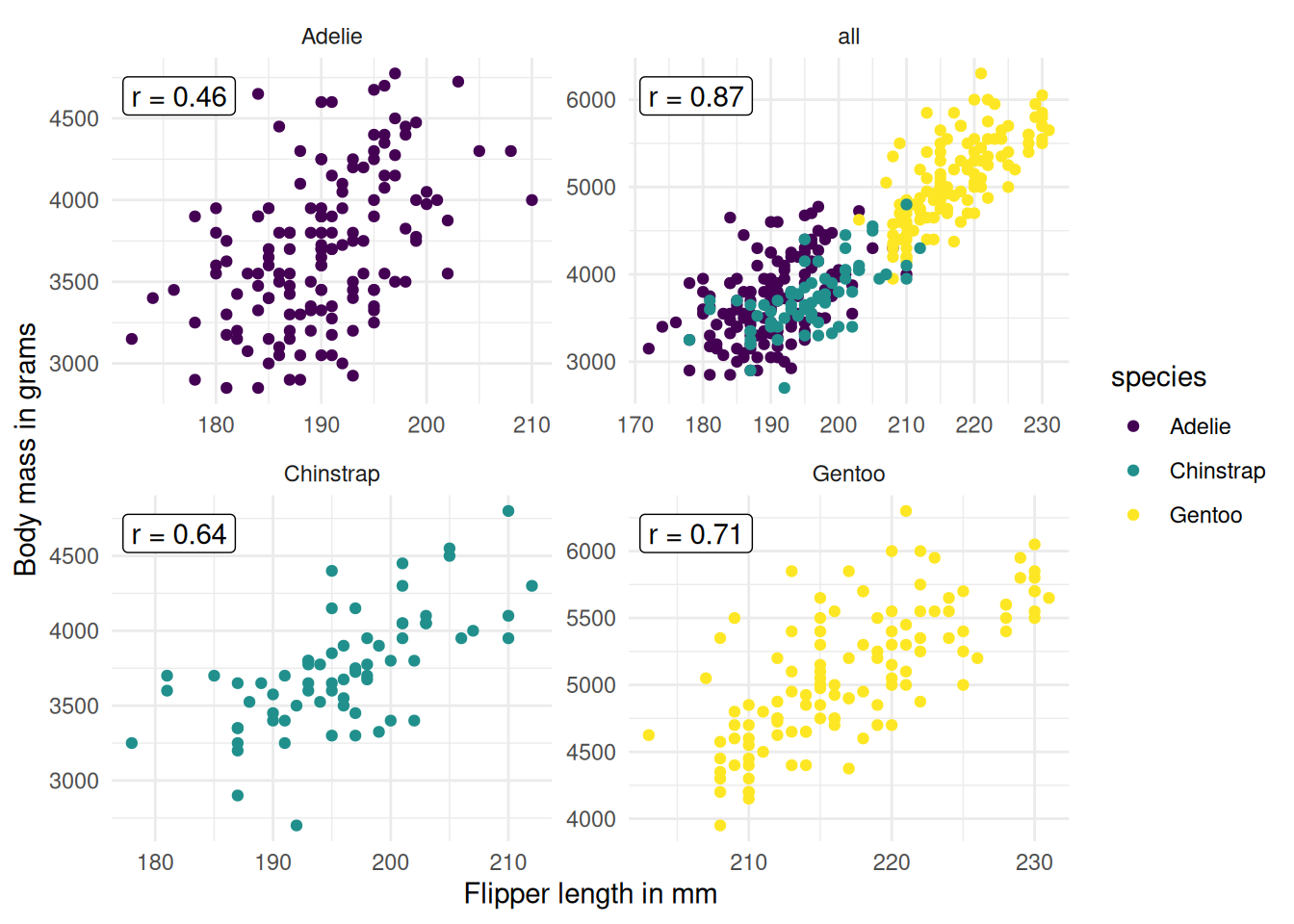
Let’s go back to the penguins. Since PFI of, e.g., body mass, is computed by permuting across all data, we mix body masses from different penguin species. But we can simply adapt PFI by splitting our data by species, and permuting for each subset separately, so that we get one PFI per feature AND species. Figure 23.3 shows that we can reduce the correlation by subsetting by species.
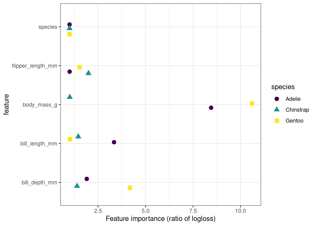
So we compute the permutation feature importance again, by species. Meaning we permute features by species, so that, for example, it can’t happen that the body mass of a heavy Gentoo is assigned to a lightweight Adelie. While grouping reduces the correlation problem, it isn’t solved, as we can see in Figure 23.3. For example, it can still happen that a Gentoo penguin with a body mass of 4000 grams gets “assigned” a flipper length of 230 mm, which produces an unrealistic data point. So still the interpretation comes with caveats. The results are displayed in Figure 23.4. A different picture emerges: Body mass is highly important for sex classification for Gentoo, less so for Adelie, and way less important for Chinstrap. Note that for the three logistic regression models it’s natural to see it as three prediction models for which we can compute separate PFIs. However, since PFI is model-agnostic, we could do the same for a random forest, which simply uses species as a feature. Or we could split into subgroups by any other variable, in theory even by variables that weren’t used by the model.
Strengths
Nice interpretation: Feature importance is the increase in model error when the feature’s information is destroyed.
Feature importance provides a highly compressed, global insight into the model’s behavior.
PFI is useful for data insights. If your goal is learning about the data, and the model is just a means to learn about the data, then PFI is great, since it relies on predictive performance (via the loss). If a feature is irrelevant for predicting the data, yet your model still uses it, then PFI will still show, in expectation, around zero importance for that feature. Other importance measures that are not based on prediction errors, like SHAP importance, will show an effect for features that are used for overfitting.
A positive aspect of using the error ratio instead of the error difference is that the feature importance measurements are comparable across different problems.
The importance measure automatically takes into account all interactions with other features. By permuting the feature, you also destroy the interaction effects with other features. This means that the permutation feature importance takes into account both the main feature effect and the interaction effects on model performance. This is also a disadvantage because the importance of the interaction between two features is included in the importance measurements of both features. This means that the feature importances do not add up to the total drop in performance, but the sum is larger. Only if there is no interaction between the features, as in a linear model, do the importances add up approximately.
Permutation feature importance does not require retraining the model. Some other methods suggest deleting a feature, retraining the model, and then comparing the model error. Since the retraining of a machine learning model can take a long time, “only” permuting a feature can save a lot of time.
Limitations
Permutation feature importance is linked to the error of the model. This is not inherently bad, but in some cases not what you need. In some cases, you might prefer to know how much the model’s output varies for a feature without considering what it means for performance. For example, you want to find out how robust your model’s output is when someone manipulates the features. In this case, you would not be interested in how much the model performance decreases when a feature is permuted, but how much of the model’s output variance is explained by each feature. Model variance (explained by the features) and feature importance correlate strongly when the model generalizes well (i.e., it does not overfit).
Feature importance doesn’t tell you how the feature influences the prediction, only how much it affects the loss. Even if you know the importance of a feature, you don’t know: Does increasing the feature increase the prediction? Are there interactions with other features? Feature importance is just a ranking.
You need access to the true outcome. If someone only provides you with the model and unlabeled data – but not the true outcome – you cannot compute the permutation feature importance.
The permutation feature importance depends on shuffling the feature, which adds randomness to the measurement. When the permutation is repeated, the results might vary greatly. Repeating the permutation and averaging the importance measures over repetitions stabilizes the measure, but increases the time of computation.
If features are correlated, the permutation feature importance can be biased by unrealistic data instances. The problem is the same as with partial dependence plots: The permutation of features produces unlikely data instances when two or more features are correlated. When they are positively correlated (like height and weight of a person) and I shuffle one of the features, I create new instances that are unlikely or even physically impossible (2 meter person weighing 30 kg for example), yet I use these new instances to measure the importance. In other words, for the permutation feature importance of a correlated feature, we consider how much the model performance decreases when we exchange the feature with values we would never observe in reality. Check if the features are strongly correlated and be careful about the interpretation of the feature importance if they are. However, pairwise correlations might not be sufficient to reveal the problem.
Another tricky thing: Adding a correlated feature can decrease the importance of the associated feature by splitting the importance between both features. Let me give you an example of what I mean by “splitting” feature importance: We want to predict the probability of rain and use the temperature at 8:00 AM of the day before as a feature along with other uncorrelated features. I train a random forest and it turns out that the temperature is the most important feature and all is well and I sleep well the next night. Now imagine another scenario in which I additionally include the temperature at 9:00 AM as a feature that is strongly correlated with the temperature at 8:00 AM. The temperature at 9:00 AM does not give me much additional information if I already know the temperature at 8:00 AM. But having more features is always good, right? I train a random forest with the two temperature features and the uncorrelated features. Some of the trees in the random forest pick up the temperature at 8:00 AM, others the temperature at 9:00 AM, again others both, and again others none. The two temperature features together have a bit more importance than the single temperature feature before, but instead of being at the top of the list of important features, each temperature is now somewhere in the middle. By introducing a correlated feature, I kicked the most important feature from the top of the importance ladder to mediocrity. On one hand, this is fine, because it simply reflects the behavior of the underlying machine learning model, here the random forest. The temperature at 8:00 AM has simply become less important because the model can now rely on the temperature at 9:00 AM measurement as well. On the other hand, it makes the interpretation of the feature importance considerably more difficult. Imagine you want to check the features for measurement errors. The check is expensive, and you decide to check only the top 3 of the most important features. In the first case, you would check the temperature; in the second case, you would not include any temperature feature just because they now share the importance. Even though the importance values might make sense at the level of model behavior, it is confusing if you have correlated features.
Software and alternatives
The iml R package was used for the examples. The R packages DALEX and vip, as well as the Python libraries alibi, eli5, scikit-learn, and rfpimp, also implement model-agnostic permutation feature importance.
An algorithm called PIMP adapts the permutation feature importance algorithm to provide p-values for the importances. Another loss-based alternative is LOFO, which omits the feature from the training data, retrains the model, and measures the increase in loss. Permuting a feature and measuring the increase in loss is not the only way to measure the importance of a feature. The different importance measures can be divided into model-specific and model-agnostic methods. The Gini importance for random forests, or standardized regression coefficients for regression models, are examples of model-specific importance measures.
A model-agnostic alternative to permutation feature importance is variance-based measures. Variance-based feature importance measures such as Sobol’s indices or functional ANOVA give higher importance to features that cause high variance in the prediction function. Also, SHAP importance has similarities to a variance-based importance measure. If changing a feature greatly changes the output, then it is important. This definition of importance differs from the loss-based definition as in the case of permutation feature importance. This is evident in cases where a model overfits. If a model overfits and uses a feature that is unrelated to the output, then the permutation feature importance would assign an importance of zero because this feature does not contribute to producing correct predictions. A variance-based importance measure, on the other hand, might assign the feature high importance as the prediction can change a lot when the feature is changed.
A good overview of various importance techniques is provided in the paper by Wei, Lu, and Song (2015).