17 Shapley Values
A prediction can be explained by assuming that each feature value of the instance is a “player” in a game where the prediction is the payout. Shapley values – a method from coalitional game theory – tell us how to fairly distribute the “payout” among the features.
Tip
Looking for a comprehensive, hands-on guide to SHAP and Shapley values? Interpreting Machine Learning Models with SHAP has you covered. With practical Python examples using the shap package, you’ll learn how to explain models ranging from simple to complex. It dives deep into the mechanics of SHAP, provides interpretation templates, and highlights key limitations, giving you the insights you need to apply SHAP confidently and effectively.
General idea
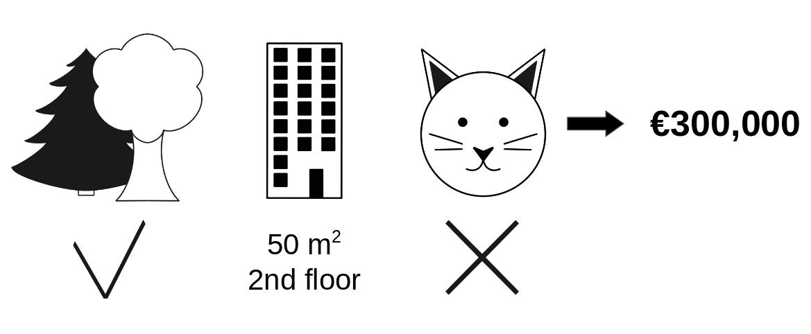
Assume the following scenario: You’ve trained a machine learning model to predict apartment prices. For a certain apartment, it predicts €300,000, and you need to explain this prediction. The apartment has an area of 50 m\(^2\), is located on the 2nd floor, has a park nearby, and cats are banned, as illustrated in Figure 17.1. The average prediction for all apartments is €310,000. Our goal is to explain how each of these feature values contributed to the prediction. How much has each feature value contributed to the prediction compared to the average prediction?
The answer is simple for linear regression models. The effect of each feature is the weight of the feature times the feature value. This only works because of the linearity of the model. For more complex models, we need a different solution. For example, LIME suggests local models to estimate effects. Another solution comes from cooperative game theory: The Shapley value, coined by Shapley (1953), is a method for assigning payouts to players depending on their contribution to the total payout. Players cooperate in a coalition and receive a certain profit from this cooperation.
Players? Game? Payout? What’s the connection to machine learning predictions and interpretability? The “game” is the prediction task for a single instance of the dataset. The “gain” is the actual prediction for this instance minus the average prediction for all instances. The “players” are the feature values of the instance that collaborate to receive the gain (= predict a certain value). In our apartment example, the feature values park-nearby, cat-banned, area-50, and floor-2nd worked together to achieve the prediction of €300,000. Our goal is to explain the difference between the actual prediction (€300,000) and the average prediction (€310,000): a difference of -€10,000.
The answer could be: The park-nearby contributed €30,000; area-50 contributed €10,000; floor-2nd contributed €0; cat-banned contributed -€50,000. The contributions add up to -€10,000, the final prediction minus the average predicted apartment price.
How do we calculate the Shapley value for one feature?
The Shapley value is the average marginal contribution of a feature value across all possible coalitions. All clear now?
Figure 17.2 shows how to calculate the marginal contribution of the cat-banned feature value when it is added to a coalition of park-nearby and area-50. We simulate that only park-nearby, cat-banned, and area-50 are in a coalition by randomly drawing another apartment from the data and using its value for the floor feature. The value floor-2nd was replaced by the randomly drawn floor-1st. Then we predict the price of the apartment with this combination (€310,000). In a second step, we remove cat-banned from the coalition by replacing it with a random value of the cat allowed/banned feature from the randomly drawn apartment. In the example, it was cat-allowed, but it could have been cat-banned again. We predict the apartment price for the coalition of park-nearby and area-50 (€320,000). The contribution of cat-banned was €310,000 - €320,000 = -€10,000. This estimate depends on the values of the randomly drawn apartment that served as a “donor” for the cat and floor feature values. We’ll get better estimates if we repeat this sampling step and average the contributions.
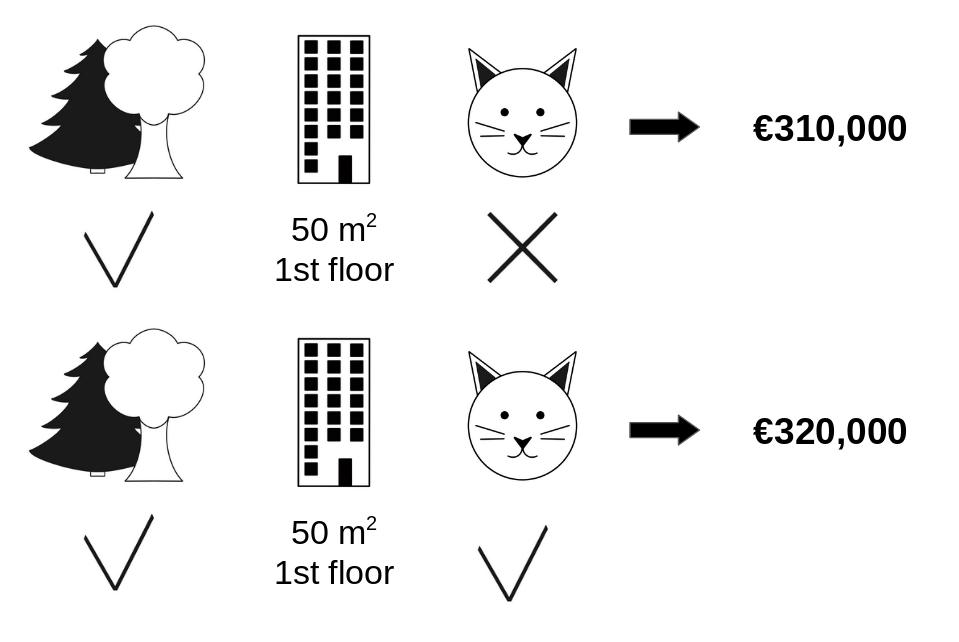
cat-banned to the prediction when added to the coalition of park-nearby and area-50.
We repeat this computation for all possible coalitions. The Shapley value is the average of all the marginal contributions to all possible coalitions. The computation time increases exponentially with the number of features. One solution to keep the computation time manageable is to compute contributions for only a few samples of the possible coalitions.
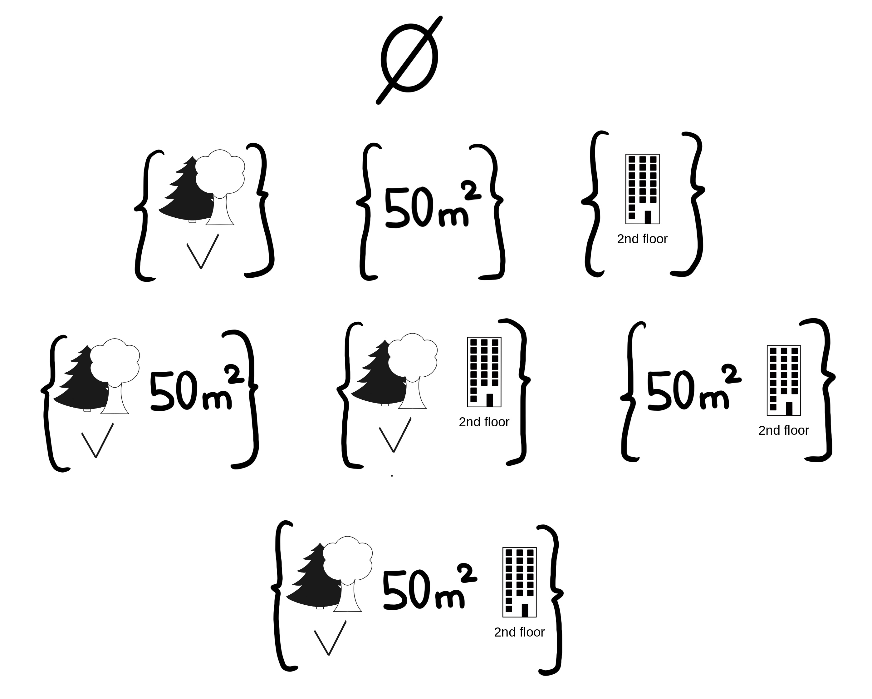
Figure 17.3 shows all coalitions of feature values that are needed to determine the exact Shapley value for cat-banned. The first row shows the coalition without any feature values. The second, third, and fourth rows show different coalitions with increasing coalition size, separated by “|”. All in all, the following coalitions are possible:
{}(empty coalition){park-nearby}{area-50}{floor-2nd}{park-nearby,area-50}{park-nearby,floor-2nd}{area-50,floor-2nd}{park-nearby,area-50,floor-2nd}
For each of these coalitions, we compute the predicted apartment price with and without the feature value cat-banned and take the difference to get the marginal contribution. The Shapley value is the (weighted) average of all marginal contributions. We replace the feature values of features that are not in a coalition with random feature values from the apartment dataset to get a prediction from the machine learning model. If we estimate the Shapley values for all feature values, we get the complete distribution of the prediction (minus the average) among the feature values.
cat-banned feature value
Examples and interpretation
The interpretation of the Shapley value for feature \(j\) is: The value of the \(j\)-th feature contributed \(\phi_j\) to the prediction of this particular instance compared to the average prediction for the dataset. The Shapley value works for both classification (if we are dealing with probabilities) and regression.
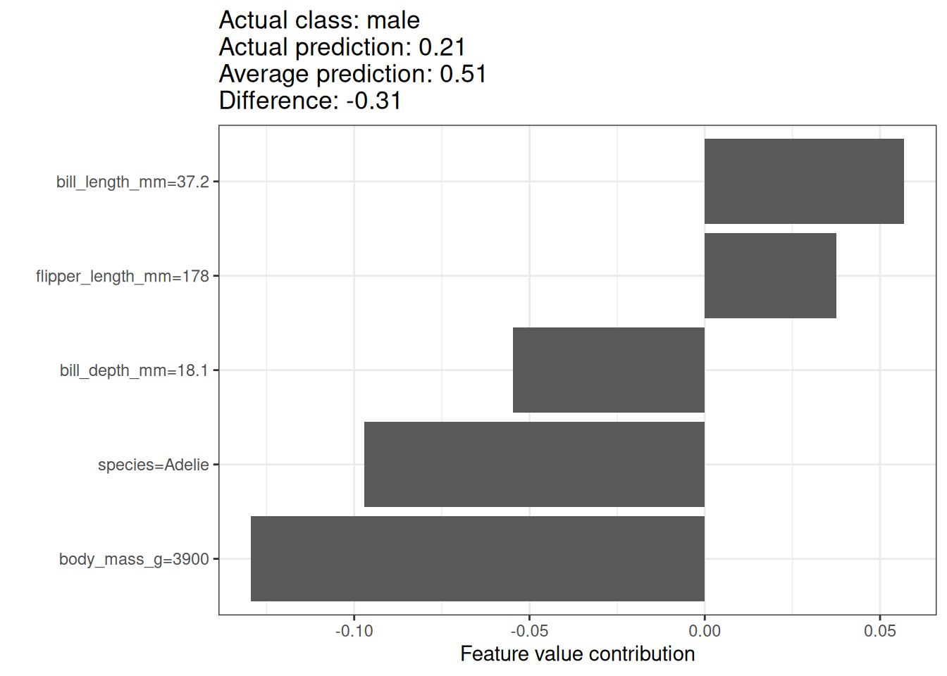
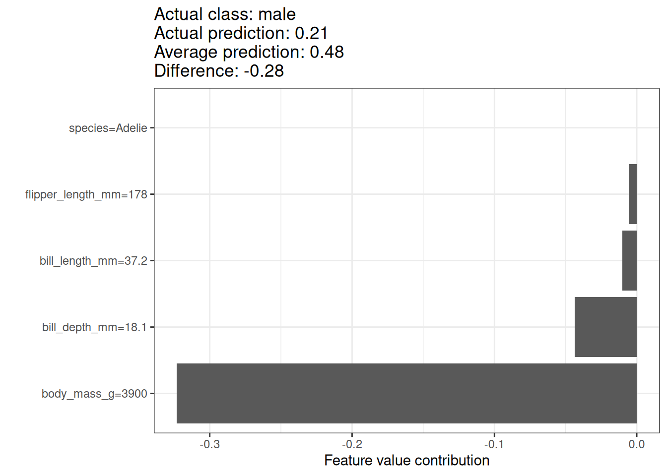
We use the Shapley value to analyze the predictions of a random forest model predicting penguin sex. Figure 17.4 shows the Shapley values for a male penguin. This penguin’s predicted P(female)=0.21 is -0.31 below the average probability for P(female) of 0.51. The bill length contributed most to the probability of being female, but most factors were (correctly) pointing to male. The sum of the contributions yields the difference between actual and average prediction (0.51).
Shapley values always need a reference dataset from which to sample the missing team members. In this case, I used all of the data points, which means all of the penguins, no matter the species. The current penguin is an Adelie penguin, and we can also compute Shapley values that only compare against other penguins of the same species. This reduces the problem of sampling and combining unrealistic values. Figure 17.5 shows also a different interpretation. When comparing our penguin with other Adelie penguins, then the reason why it has a low probability of being female is its body weight.
Pick the reference data
Shapley value interpretation is always in reference to the dataset that was used for replacing values for absent players. Make sure to pick a meaningful reference dataset.
For the bike rental dataset, we also train a random forest to predict the number of rented bikes for a day, given weather and calendar information. The explanations created for the random forest prediction of a particular day are shown in Figure 17.6.
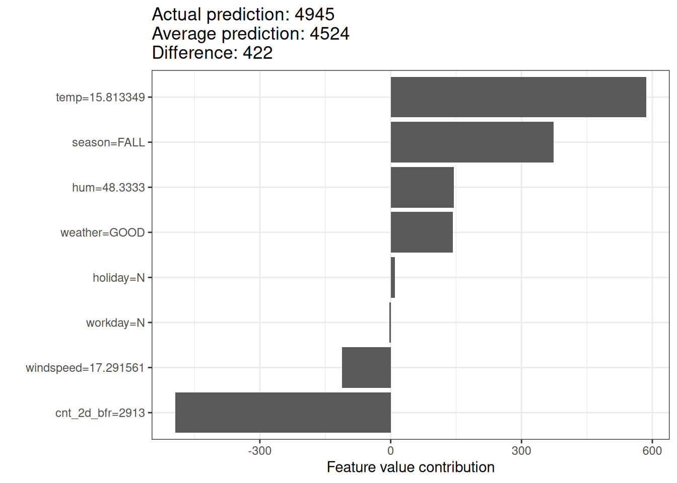
With a predicted 5028 rental bikes, this day is 505 below the average prediction of 4522. The temperature and humidity had the largest positive contributions. The low count two days before had the largest negative contribution. The sum of Shapley values yields the difference of actual and average prediction (505).
Shapley values are not counterfactuals
Be careful to interpret the Shapley value correctly: The Shapley value is the average contribution of a feature value to the prediction in different coalitions. The Shapley value is NOT the difference in prediction when we remove the feature from the model.
Shapley value theory
This section goes deeper into the definition and computation of the Shapley value for the curious reader. Skip this section and go directly to “Strengths and Limitations” if you are not interested in the technical details.
We are interested in how each feature affects the prediction of a data point. In a linear model, it’s easy to calculate the individual effects. Here’s what a linear model prediction looks like for one data instance:
\[\hat{f}(\mathbf{x})=\beta_0+\beta_{1}x_{1}+\ldots+\beta_{p}x_{p}\]
where \(\mathbf{x}\) is the instance for which we want to compute the contributions. Each \(x_j\) is a feature value, with \(j = 1,\ldots,p\). The \(\beta_j\) is the weight corresponding to feature \(j\).
The contribution \(\phi_j\) of the \(j\)-th feature to the prediction \(\hat{f}(\mathbf{x})\) is:
\[\phi_j(\hat{f})=\beta_{j}x_j-\beta_{j}\mathbb{E}[X_{j}]\]
where \(\beta_j \mathbb{E}[X_{j}]\) is the mean effect estimate for feature \(j\). The contribution is the difference between the feature effect and the average effect. Nice! Now we know how much each feature contributed to the prediction. If we sum all the feature contributions for one instance, the result is the following:
\[\begin{align*} \sum_{j=1}^{p}\phi_j(\hat{f})=&\sum_{j=1}^p(\beta_{j}x_j- \beta_{j} \mathbb{E}[X_{j}]) \\ =&(\beta_0+\sum_{j=1}^p\beta_{j}x_j)-(\beta_0+\sum_{j=1}^p \beta_{j} \mathbb{E}[X_{j}]) \\ =&\hat{f}(\mathbf{x})-\mathbb{E}[\hat{f}(\mathbf{X})] \end{align*}\]
This is the predicted value for the data point \(\mathbf{x}\) minus the average predicted value. Feature contributions can be negative.
Can we do the same for any type of model? It would be great to have this as a model-agnostic tool. Since we usually do not have similar weights in other model types, we need a different solution.
Help comes from unexpected places: cooperative game theory. The Shapley value is a solution for computing feature contributions for single predictions for any machine learning model.
Definition
The Shapley value is defined via a value function \(val\) of players in \(S\).
The Shapley value of a feature value is its contribution to the payout, weighted and summed over all possible feature value combinations:
\[\phi_j(val)=\sum_{S\subseteq\{1,\ldots,p\} \setminus \{j\}}\frac{|S|!\left(p-|S|-1\right)!}{p!}\left(val\left(S\cup\{j\}\right)-val(S)\right)\]
where \(S\) is a subset of the features used in the model, \(\mathbf{x}\) is the vector of feature values of the instance to be explained, and \(p\) is the number of features. \(val_{\mathbf{x}}(S)\) is the prediction for feature values in set \(S\) that are marginalized over features \(X_C\), which are all the features not included in \(S\) (\(S \cap C = \emptyset\) and \(S \cup C = \{1, \ldots, p\}\)):
\[val_{\mathbf{x}}(S)=\int\hat{f}(x_{1},\ldots,x_{p})d\mathbb{P}_{X_C}-\mathbb{E}[\hat{f}(\mathbf{X})]\]
You actually perform multiple integrations for each feature that is not contained in \(S\). A concrete example: The machine learning model works with 4 features \(X_1\), \(X_2\), \(X_3\), and \(X_4\), and we evaluate the prediction for the coalition \(S\) consisting of feature values \(x_1\) and \(x_3\):
\[val_{\mathbf{x}}(S)=val_{\mathbf{x}}(\{1,3\})=\int_{\mathbb{R}}\int_{\mathbb{R}}\hat{f}(x_{1},X_{2},x_{3},X_{4})d\mathbb{P}_{X_2X_4}-\mathbb{E}[\hat{f}(\mathbf{X})]\]
This looks similar to the feature contributions in the linear model!
Don’t get confused by the many uses of the word “value”
The feature value is the numerical or categorical value of a feature and instance; the Shapley value is the feature contribution to the prediction; the value function is the payout function for coalitions of players (feature values).
The Shapley value is the only attribution method that satisfies the properties Efficiency, Symmetry, Dummy, and Additivity, which together can be considered a definition of a fair payout.
Efficiency The feature contributions must add up to the difference of prediction for \(\mathbf{x}\) and the average.
\[\sum\nolimits_{j=1}^p\phi_j=\hat{f}(\mathbf{x})-\mathbb{E}[\hat{f}(\mathbf{X})]\]
Symmetry The contributions of two feature values \(j\) and \(k\) should be the same if they contribute equally to all possible coalitions. If
\[val(S \cup \{j\})=val(S\cup\{k\})\]
for all
\[S\subseteq\{1,\ldots, p\} \setminus \{j,k\}\]
then
\[\phi_j=\phi_{k}\]
Dummy A feature \(j\) that does not change the predicted value – regardless of which coalition of feature values it is added to – should have a Shapley value of 0. If
\[val(S\cup\{j\})=val(S)\]
for all
\[S\subseteq\{1,\ldots,p\}\]
then
\[\phi_j=0\]
Additivity For a game with combined payouts \(val + val^+\) the respective Shapley values are as follows:
\[\phi_j+\phi_j^{+}\]
Suppose you trained a random forest, which means that the prediction is an average of many decision trees. The Additivity property guarantees that for a feature value, you can calculate the Shapley value for each tree individually, average them, and get the Shapley value for the feature value for the random forest.
Intuitive understanding of Shapley values
The feature values enter a room in random order. All feature values in the room participate in the game (= contribute to the prediction). The Shapley value of a feature value is the average change in the prediction that the coalition already in the room receives when the feature value joins them.
Estimating Shapley values
All possible coalitions (sets) of feature values have to be evaluated with and without the \(j\)-th feature to calculate the exact Shapley value. For more than a few features, the exact solution to this problem becomes problematic as the number of possible coalitions exponentially increases as more features are added. Štrumbelj and Kononenko (2014) proposed an approximation with Monte-Carlo sampling:
\[\hat{\phi}_{j} = \frac{1}{M}\sum_{m=1}^M\left(\hat{f}(\mathbf{x}^{(m)}_{+j}) - \hat{f}(\mathbf{x}^{(m)}_{-j})\right)\]
where \(\hat{f}(\mathbf{x}^{(m)}_{+j})\) is the prediction for \(\mathbf{x}\), but with a random number of feature values replaced by feature values from a random data point \(\mathbf{z}\), except for the respective value of feature \(j\). The feature vector \(\mathbf{x}^{(m)}_{-j}\) is almost identical to \(\mathbf{x}^{(m)}_{+j}\), but the value \(x^{(m)}_j\) is also taken from the sampled \(\mathbf{z}\). Each of these \(M\) new instances is a kind of “Frankenstein’s Monster” assembled from two instances. Note that in the following algorithm, the order of features is not actually changed – each feature remains at the same vector position when passed to the predict function. The order is only used as a “trick” here: By giving the features a new order, we get a random mechanism that helps us put together the “Frankenstein’s Monster.” For features that appear left of the feature \(X_j\), we take the values from the original observations, and for the features on the right, we take the values from a random instance.
Approximate Shapley estimation for a single feature value:
- Output: Shapley value for the value of the \(j\)-th feature
- Required: Number of iterations \(M\), instance of interest \(\mathbf{x}\), feature index \(j\), data matrix \(\mathbf{X}\), and machine learning model \(f\)
- For all \(m = 1,\ldots,M\):
- Draw random instance \(\mathbf{z}\) from the data matrix \(\mathbf{X}\)
- Choose a random permutation \(\mathbf{o}\) of the feature values
- Order instance \(\mathbf{x}\): \(\mathbf{x}_{\mathbf{o}}=(x_{(1)},\ldots,x_{(j)},\ldots,x_{(p)})\)
- Order instance \(\mathbf{z}\): \(\mathbf{z}_{\mathbf{o}}=(z_{(1)},\ldots,z_{(j)},\ldots,z_{(p)})\)
- Construct two new instances
- With \(j\): \(\mathbf{x}_{+j}=(x_{(1)},\ldots,x_{(j-1)},x_{(j)},z_{(j+1)},\ldots,z_{(p)})\)
- Without \(j\): \(\mathbf{x}_{-j}=(x_{(1)},\ldots,x_{(j-1)},z_{(j)},z_{(j+1)},\ldots,z_{(p)})\)
- Compute marginal contribution: \(\phi_j^{(m)}=\hat{f}(\mathbf{x}_{+j})-\hat{f}(\mathbf{x}_{-j})\)
- Compute Shapley value as the average: \(\phi_j(\mathbf{x}) = \frac{1}{M}\sum_{m=1}^M\phi_j^{(m)}\)
Reduce sample size for speed
Consider using a smaller sample size \(M\) when estimating Shapley values to reduce computation time, but beware of increased variance in the estimate.
The procedure has to be repeated for each of the features to get all Shapley values. In the SHAP chapter, we will see other efficient ways to estimating Shapley values.
Strengths
The difference between the prediction and the average prediction is fairly distributed among the feature values of the instance – the Efficiency property of Shapley values. This property distinguishes the Shapley value from other methods such as LIME. LIME does not guarantee that the prediction is fairly distributed among the features. The Shapley values deliver a full explanation.
The Shapley value allows contrastive explanations. Instead of comparing a prediction to the average prediction of the entire dataset, you could compare it to a subset or even to a single data point. This contrastiveness is also something that local models like LIME do not have.
The Shapley value is the only explanation method with a solid theory. The axioms – efficiency, symmetry, dummy, additivity – give the explanation a reasonable foundation. Methods like LIME assume linear behavior of the machine learning model locally, but there is no theory as to why this should work.
Limitations
The Shapley value requires a lot of computing time. In 99.9% of real-world problems, only the approximate solution is feasible. An exact computation of the Shapley value is computationally expensive because there are 2k possible coalitions of the feature values and the “absence” of a feature has to be simulated by drawing random instances, which increases the variance for the estimate of the Shapley values estimation. The exponential number of the coalitions is dealt with by sampling coalitions and limiting the number of iterations M. Decreasing M reduces computation time, but increases the variance of the Shapley value. There’s no good rule of thumb for the number of iterations M. M should be large enough to accurately estimate the Shapley values, but small enough to complete the computation in a reasonable time. It should be possible to choose M based on Chernoff bounds, but I have not seen any paper on doing this for Shapley values for machine learning predictions.
The Shapley value can be misinterpreted. The Shapley value of a feature value is not the difference of the predicted value after removing the feature from the model training. The interpretation of the Shapley value is: Given the current set of feature values, the contribution of a feature value to the difference between the actual prediction and the mean prediction is the estimated Shapley value.
Shapley value explanations are not to be interpreted as local in the sense of gradients or neighborhood. (Bilodeau et al. 2024) For example, a positive Shapley value doesn’t mean that increasing the feature would increase the prediction. Instead, the Shapley value has to be interpreted with respect to the reference dataset that was used for the estimation. That’s why I would also recommend pairing Shapley values with, for example, ceteris paribus plots or ICE plots, so you get the full picture.
Combine with ceteris paribus and ICE
Pair Shapley values with ceteris paribus or ICE plots to get a sense of local sensitivity to feature changes.
The Shapley value is the wrong explanation method if you seek sparse explanations (explanations that contain few features). Explanations created with the Shapley value method use all the features. Humans prefer selective explanations, such as those produced by LIME. LIME might be the better choice for explanations laypersons have to deal with. Another solution is SHAP introduced by Lundberg and Lee (2017), which is based on the Shapley value but can also provide explanations with few features.
The Shapley value returns a simple value per feature, but no prediction model like LIME. This means it cannot be used to make statements about changes in prediction for changes in the input, such as: “If I were to earn €300 more a year, my credit score would increase by 5 points.”
Like many other permutation-based interpretation methods, the Shapley value method suffers from inclusion of unrealistic data instances when features are correlated. To simulate that a feature value is missing from a coalition, we marginalize the feature. This is achieved by sampling values from the feature’s marginal distribution. This is fine as long as the features are independent. When features are dependent, then we might sample feature values that do not make sense for this instance. But we would use those to compute the feature’s Shapley value. One solution might be to permute correlated features together and get one mutual Shapley value for them. Another adaptation is conditional sampling: Features are sampled conditional on the features that are already in the team. While conditional sampling fixes the issue of unrealistic data points, a new issue is introduced: The resulting values are no longer the Shapley values to our game, since they violate the symmetry axiom, as found out by Sundararajan and Najmi (2020) and further discussed by Janzing, Minorics, and Blöbaum (2020).
Software and alternatives
Shapley values are implemented in both the iml and fastshap packages for R. In Julia, you can use Shapley.jl.
SHAP, an alternative estimation method and ecosystem for Shapley values, is presented in the next chapter.
Another approach is called breakDown, which is implemented in the breakDown R package (Staniak and Biecek 2018). BreakDown also shows the contributions of each feature to the prediction but computes them step by step. Let’s reuse the game analogy: We start with an empty team, add the feature value that would contribute the most to the prediction and iterate until all feature values are added. How much each feature value contributes depends on the respective feature values that are already in the “team”, which is the big drawback of the breakDown method. It’s faster than the Shapley value method, and for models without interactions, the results are the same.