4 Methods Overview
This chapter provides an overview of interpretability approaches. The goal is to give you a map so that when you dive into the individual models and methods, you can see the forest for the trees. Figure 4.1 provides a taxonomy of the different approaches.
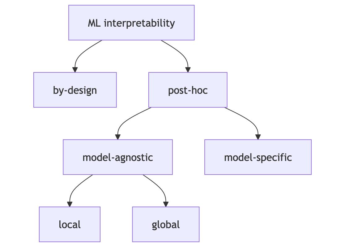
In general, we can distinguish between interpretability by design and post-hoc interpretability. Interpretability by design means that we train inherently interpretable models, such as using logistic regression instead of a random forest. Post-hoc interpretability means that we use an interpretability method after the model is trained. Post-hoc interpretation methods can be model-agnostic, such as permutation feature importance, or model-specific, such as analyzing the features learned by a neural network. Model-agnostic methods can be further divided into local methods which focus on explaining individual predictions, and global methods which focus on datasets. This book focuses on post-hoc model-agnostic methods but also covers basic models that are interpretable by design and model-specific methods for neural networks.
Let’s look at each category of interpretability and also discuss strengths and weaknesses as they relate to your interpretation goals.
Interpretable models by design
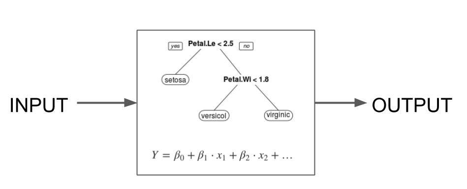
Interpretability by design is decided on the level of the machine learning algorithm. If you want a machine learning algorithm that produces interpretable models, the algorithm has to constrain the search of models to those that are interpretable. The simplest example is linear regression: When you use ordinary least squares to fit/train a linear regression model, you are using an algorithm that will produce find models that are linear in the input features. Models that are interpretable by design are also called intrinsically or inherently interpretable models, see Figure 4.2.
This book covers the most basic interpretability by design approaches:
- Linear regression: Fit a linear model by minimizing the sum of squared errors.
- Logistic regression: Extend linear regression for classification using a nonlinear transformation.
- Linear model extensions: Add penalties, interactions, and nonlinear terms for more flexibility.
- Decision trees: Recursively split data to create tree-based models.
- Decision rules: Extract if-then rules from data.
- RuleFit: Combine tree-based rules with Lasso regression to learn sparse rule-based models.
There are many more approaches to interpretable models, ranging from extensions of these basic approaches to very specialized approaches. Including all of them would be impossible, so I have focused on the basic ones. Here are some examples of other interpretable-by-design approaches:
- Prototype-based neural networks for image classification, called ProtoViT (Ma et al. 2024). These neural networks are trained so that the image classification is a weighted sum of prototypes (special images from the training data) and sub-prototypes.
- Yang et al. (2024) proposed inherently interpretable tree ensembles which are boosted trees (e.g., with XGBoost) with adjusted hyperparameters, such as low maximum tree depth, a different representation where feature effects are sorted into main effects and interactions, and pruning of effects. This approach mixes both interpretability by design and post-hoc interpretability.
- Model-based boosting is an additive modeling framework. The trained model is a weighted sum of linear effects, splines, tree stumps, and other so-called weak learners (Bühlmann and Hothorn 2007).
- Generalized additive models with automatic interaction detection (Caruana et al. 2015).
But how interpretable are intrinsically interpretable models? Approaches to interpretable models differ wildly and so do their interpretation. Let’s talk about the scope of interpretability, which helps us sort the approaches:
- The model is entirely interpretable. Example: a small decision tree can be visualized and understand easily. Or a linear regression model with not too many coefficients. “Entirely interpretable” is a tough requirement, and again a bit fuzzy at the same time. My stance is that the term entirely interpretable may only be used for the simplest of models such as very sparse linear regression or very short trees, if at all.
- Parts of the model are interpretable. While a regression model with hundreds of features may not be “entirely interpretable”, we can still interpret the individual coefficients associated with the features. Or if you have a huge decision list, you can still inspect individual rules.
- The model predictions are interpretable. Some approaches allow us to interpret individual predictions. Let’s say you would develop a \(k\)-nearest neighbor-like machine learning algorithm, but for images. To classify an image, take the \(k\) most similar images and return the most common class. A prediction is fully explained by showing the \(k\) similar images. Or for decision trees, a prediction is explained by returning the decision list that led to the prediction.
When exploring a new interpretability approach, assess the scope of interpretability. Ask at which levels (entirely interpretable, partially interpretable, or interpretable predictions) the approach operates.
Models that are interpretable by design are usually easier to debug and improve because we get insights into their inner workings.
Interpretability by design also shines when it comes to justifying models and outputs, as they often faithfully explain how predictions were made. They also tend to make it easier to check with domain experts that the models are consistent with domain knowledge. Many data-driven fields already have established (interpretable) modeling approaches, such as logistic regression in medical research.
When it comes to discovering insights, interpretable models are a mixed bag. They make it easy to extract insights about the models themselves. But it gets trickier when it comes to data insights because of the need for a theoretical link between model structure and data. To interpret the model in place of the data, you have to assume that the model structure reflects the world – something statisticians work very hard on and need a lot of assumptions for. But what if there is a model with better predictive performance? You would have to argue why the interpretable model represents the data correctly, even though its predictive performance is inferior. In addition, there are often multiple models with similar performance but different interpretations, which makes our job more difficult. This is called the Rashomon effect. The problem with this model multiplicity is that it makes it very unclear which model to interpret.
The Japanese movie Rashomon from 1950 tells four different versions of a murder story. While each version can explain the events equally well, they are incompatible with each other. This phenomenon was named the Rashomon effect.
Post-hoc interpretability
Post-hoc methods are applied after the model has been trained. These methods can be either model-agnostic or model-specific:
- Model-agnostic: We ignore what’s inside the model and only analyze how the model output changes with respect to changes in the feature inputs. For example, permuting a feature and measuring how much the model error increases.
- Model-specific: We analyze parts of the model to better understand it. This can be analyzing which types of images a neuron in a neural network responds to the most, or the Gini importance in random forests.
Model-agnostic post-hoc methods
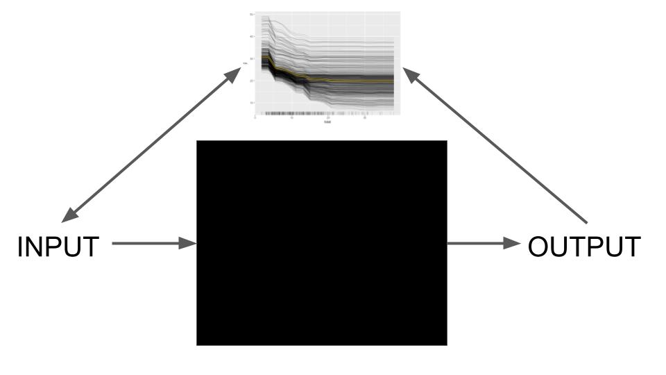
Model-agnostic methods work by the SIPA principle: sample from the data, perform an intervention on the data, get the predictions for the manipulated data, and aggregate the results (Scholbeck et al. 2020). An example is permutation feature importance: We take a data sample, intervene on the data by permuting it, get the model predictions, and compute the model error again and compare it to the original loss (aggregation). What makes these methods model-agnostic is that they don’t need to “look inside” the model, like reading out coefficients or weights, as visualized in Figure 4.3.
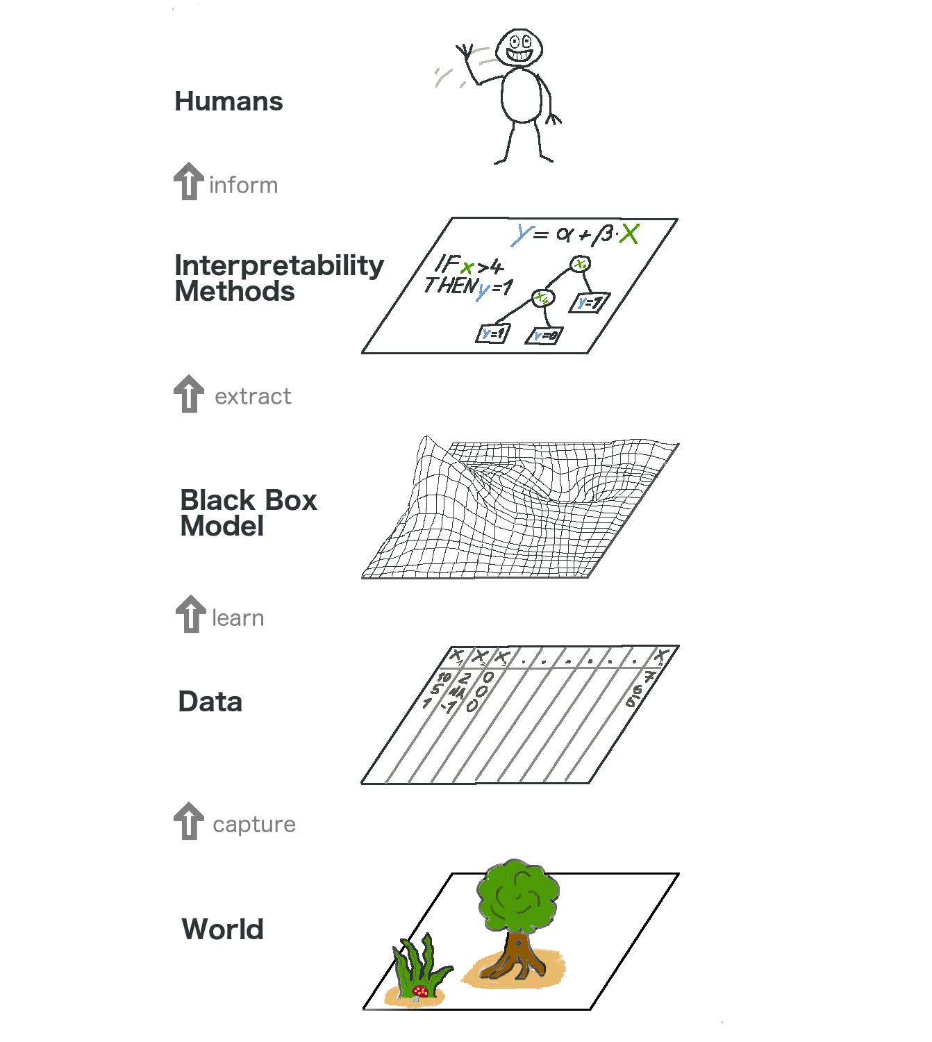
Model-agnostic interpretation separates the model interpretation from the model training. Looking at this from a higher level, the modeling process gains another layer: It starts with the world, which we capture in the form of data, from which we learn a model. On top of that model, we have interpretability methods for humans to consume. See Figure 4.4. For model-agnostic methods, we have this separation, while for interpretability by design, we have model and interpretability layers merged into one.
Separating the explanations from the machine learning model (= model-agnostic interpretation methods) has some advantages (Ribeiro, Singh, and Guestrin 2016). The biggest strength is flexibility in both the choice of model and the choice of interpretation method. For example, if you’re visualizing feature effects of an XGBoost model with the partial dependence plot (PDP), you can even change the underlying model and still use the same type of interpretation. Or, if you no longer like the PDP, you can use accumulated local effects (ALE) without having to change the underlying XGBoost model. But if you are using a linear regression model and interpret the coefficients, switching to a rule-based classifier will also change the means of interpretation. Some model-agnostic methods even give you flexibility in the feature representation used to create the explanations: For example, you can create explanations based on image patches instead of pixels when explaining image classifier outputs.
Model-agnostic interpretation methods can be further divided into local and global methods. Local methods aim to explain individual predictions, while global methods describe how features affect predictions on average.
Local model-agnostic post hoc methods
Local interpretation methods explain individual predictions. Approaches in this category are quite diverse:
- Ceteris paribus plots show how changing a feature changes a prediction.
- Individual conditional expectation curves show how changing one feature changes the prediction of multiple data points.
- Local surrogate models (LIME) explain a prediction by replacing the complex model with a locally interpretable model.
- Scoped rules (anchors) are rules that describe which feature values “anchor” a prediction, meaning that no matter how many of the other features you change, the prediction remains fixed.
- Counterfactual explanations explain a prediction by examining which features would need to be changed to achieve a desired prediction.
- Shapley values fairly assign the prediction to individual features.
- SHAP is a computation method for Shapley values but also suggests global interpretation methods based on combinations of Shapley values across the data.
LIME and Shapley values (and SHAP) are attribution methods that explain a data point’s prediction as the sum of feature effects. Other methods, such as ceteris paribus and ICE, focus on individual features and how sensitive the prediction function is to those features. Methods such as counterfactual explanations and anchors fall somewhere in the middle, relying on a subset of the features to explain a prediction.
For model debugging, local methods provide a “zoomed in” view that can be useful for understanding edge cases or studying unusual predictions. For example, you can look at explanations for the prediction with the worst prediction error and see if it’s just a difficult data point to predict, or if maybe your model isn’t good enough, or the data point is mislabeled. Beyond that, it’s the global model-agnostic methods that are more useful for model improvements.
When it comes to using local interpretation methods to justify individual predictions, the usefulness is mixed: Methods such as ceteris paribus and counterfactual explanations can be very useful for justifying model predictions because they faithfully reflect the raw model predictions. Attribution methods like SHAP or LIME are themselves a kind of “model” (or at least more complex estimates) on top of the model being explained and therefore may not be as suitable for high-stakes justification purposes (Rudin 2019).
Local methods can be useful for data insights. Attribution methods such as Shapley values work with a reference dataset and therefore allow comparing the current prediction with different subsets, allowing different questions to be asked. In general, the usefulness of model-agnostic interpretation for both local and global methods depends on model performance. Ceteris paribus plots and ICE are also useful for model insights.
Global model-agnostic post-hoc methods
Global methods describe the average behavior of a machine learning model across a dataset. In this book, you will learn about the following model-agnostic global interpretation techniques:
- The partial dependence plot is a feature effect method.
- Accumulated local effect plots also visualize feature effects, designed also for correlated features.
- Feature interaction (H-statistic) quantifies the extent to which the prediction is the result of joint effects of the features.
- Functional decomposition is a central idea of interpretability and a technique for decomposing prediction functions into smaller parts.
- Permutation feature importance measures the importance of a feature as an increase in loss when the feature is permuted.
- Leave one feature out (LOFO) removes a feature and measures the increase in loss after retraining the model without that feature.
- Surrogate models replace the original model with a simpler model for interpretation.
- Prototypes and criticisms are representative data points of a distribution and can be used to improve interpretability.
Two broad categories within global model-agnostic methods are feature effects and feature importance. Feature effects (PDP, ALE, H-statistic, decomposition) are about showing the relationship between inputs and outputs. Feature importance (PFI, LOFO, SHAP importance, …) is about ranking the features by importance, where importance is defined differently by each of the methods.
Since global interpretation methods describe average behavior, they are particularly useful when the modeler wants to debug a model. In particular, LOFO is related to feature selection methods and is particularly useful for model improvement.
To justify the models to stakeholders, global interpretation methods can provide some broad strokes such as which features were relevant. You can also use global methods in combination with inherently interpretable models. For example, while decision rule lists make it easy to justify individual predictions, you may also want to justify the model itself by showing which features were important overall.
Global methods are often expressed as expected values based on the distribution of the data. For example, the partial dependence plot, a feature effect plot, is the expected prediction when all other features are marginalized out. This is what makes these methods so useful for understanding the general mechanisms in the data. My colleagues and I wrote papers about the PDP and PFI, and how they can be used to infer properties about the data (Molnar et al. 2023; Freiesleben et al. 2024).
By applying global methods to subsets of your data, you can turn global methods into “group-wise” or “regional” methods. We will see this in action in the examples in this book.
Model-specific post-hoc methods
As the name implies, post-hoc model-specific methods are applied after model training but only work for specific machine learning models, as visualized in Figure 4.5. There are many such examples, ranging from Gini importance for random forests to computing odds ratios for logistic regression. This book focuses on post-hoc interpretation methods for neural networks.
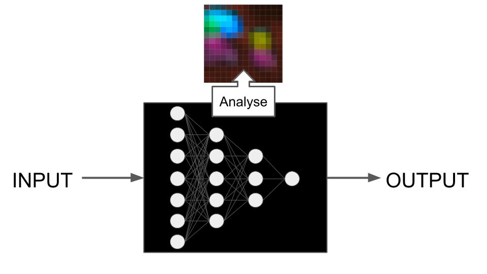
To make predictions with a neural network, the input data is passed through many layers of multiplication with the learned weights and through non-linear transformations. A single prediction can involve millions of multiplications, depending on the architecture of the neural network. There’s no chance that we humans can follow the exact mapping from data input to prediction. We would have to consider millions of weights interacting in complex ways to understand a neural network’s prediction. To interpret the behavior and predictions of neural networks, we need specific interpretation methods. Neural networks are an interesting target for interpretation because neural networks learn features and concepts in their hidden layers. Also, we can leverage their gradients for computationally efficient methods.
The neural network part covers the following techniques that answer different questions:
- Learned Features: What features did the neural network learn?
- Saliency Maps: How did each pixel contribute to a particular prediction?
- Concepts: Which concepts did the neural network learn?
- Adversarial Examples: How can we fool the neural network?
- Influential Instances: How influential was a training data point for a given prediction?
In general, the biggest strength of model-specific methods is the ability to learn about the models themselves. This can also help improve the model and justify it to others. When it comes to data insights, model-specific methods have similar problems as intrinsically interpretable models: They need a theoretical justification for why the model interpretation reflects the data.
The lines are blurred
I’ve presented different neat categories. But in reality, the lines between by design and post hoc are blurry. Just a few examples:
- Is logistic regression an intrinsically interpretable model? You have to post-process the coefficients to interpret the odds ratios. And if you want to interpret the model effects at the level of probabilities, you have to compute marginal effects, which can definitely be seen as a post-hoc interpretation method (which can also be applied to other models).
- Boosted tree ensembles are not considered to be interpretable. But if you set the maximum tree depth to 1, you get boosted tree stumps, which gives you something like a generalized additive model.
- To explain a linear regression prediction, you can multiply each feature value with its coefficient. These are then called effects. In addition, you can subtract from each effect the average effect from the data. If you do these things, you have computed Shapley values, which are typically considered to be model-agnostic.
The moral of the story. Interpretability is a fuzzy concept. Embrace that fuzziness, don’t get too attached to one approach, but feel free to mix and match approaches.