7 Logistic Regression
Logistic regression models the probabilities for classification problems with two possible outcomes. It’s an extension of the linear regression model for class outcomes.1
Tip
Just looking for the correct interpretation of logistic regression models? Save yourself time and headaches (log odds, anyone?) and check out my logistic regression interpretation cheat sheet.
Don’t use linear regression for classification
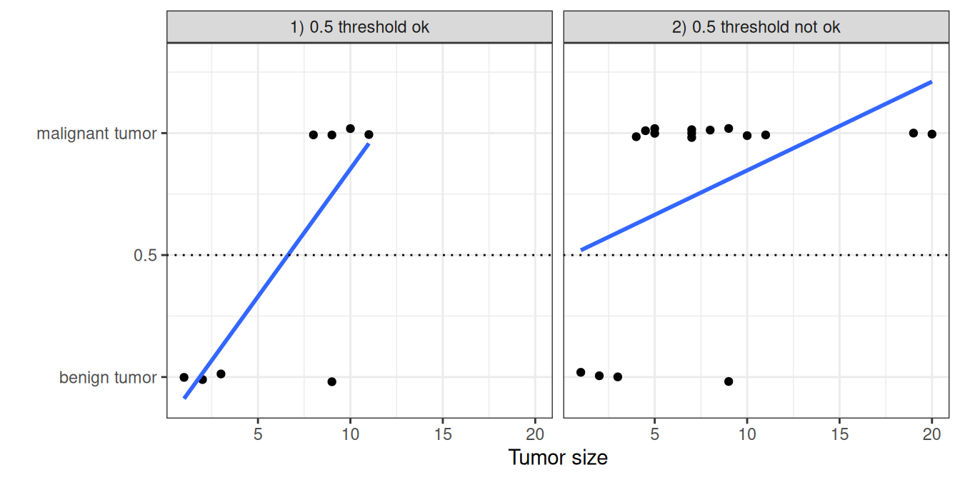
The linear regression model can work well for regression, but fails for classification. Why is that? In the case of two classes, you could label one of the classes with 0 and the other with 1 and use linear regression. Technically, it works, and most linear model programs will spit out weights for you. But there are a few problems with this approach: A linear model does not output probabilities, but it treats the classes as numbers (0 and 1) and fits the best hyperplane (for a single feature, it’s a line) that minimizes the distances between the points and the hyperplane. So it simply interpolates between the points, and you cannot interpret it as probabilities.
A linear model also extrapolates and gives you values below zero and above one. This is a good sign that there might be a smarter approach to classification.
Since the predicted outcome is not a probability, but a linear interpolation between points, there is no meaningful threshold at which you can distinguish one class from the other, as illustrated in Figure 7.1. A good explanation of this issue has been given on Stackoverflow.
Linear models don’t extend to classification problems with multiple classes. You would have to start labeling the next class with 2, then 3, and so on. The classes might not have any meaningful order, but the linear model would force a weird structure on the relationship between the features and your class predictions. The higher the value of a feature with a positive weight, the more it contributes to the prediction of a class with a higher number, even if classes that happen to get a similar number are not closer than other classes.
Theory
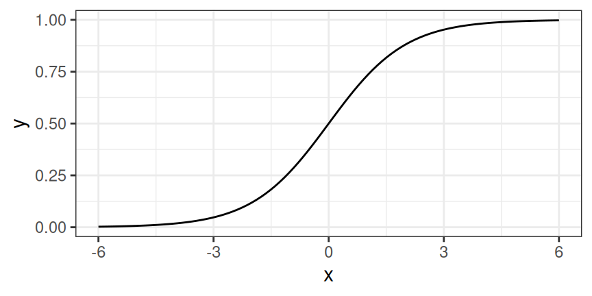
A solution for classification is logistic regression. Instead of fitting a straight line or hyperplane, the logistic regression model uses the logistic function to squeeze the output of a linear equation between 0 and 1. The logistic function is defined as:
\[\text{logistic}(\mathbf{z})=\frac{1}{1+\exp(-\mathbf{z})}\]
The logistic function is visualized in Figure 7.2.
The step from linear regression to logistic regression is kind of straightforward. In the linear regression model, we have modeled the relationship between outcome and features with a linear equation:
\[\hat{y}^{(i)}=\beta_{0}+\beta_{1}x^{(i)}_{1}+\ldots+\beta_{p}x^{(i)}_{p}\]
For classification, we prefer probabilities between 0 and 1, so we wrap the right side of the equation into the logistic function. This forces the output to assume only values between 0 and 1.
\[\mathbb{P}(Y^{(i)}=1)= \text{logistic}(\mathbf{x}^{(i)T} \boldsymbol{\beta}) = \frac{1}{1 + \exp(-(\beta_{0} + \beta_{1} x^{(i)}_{1} + \ldots + \beta_{p} x^{(i)}_{p}))}\]
Let’s revisit the tumor size example again. But instead of the linear regression model, we use the logistic regression model and get a much better fitting curve, see Figure 7.3.
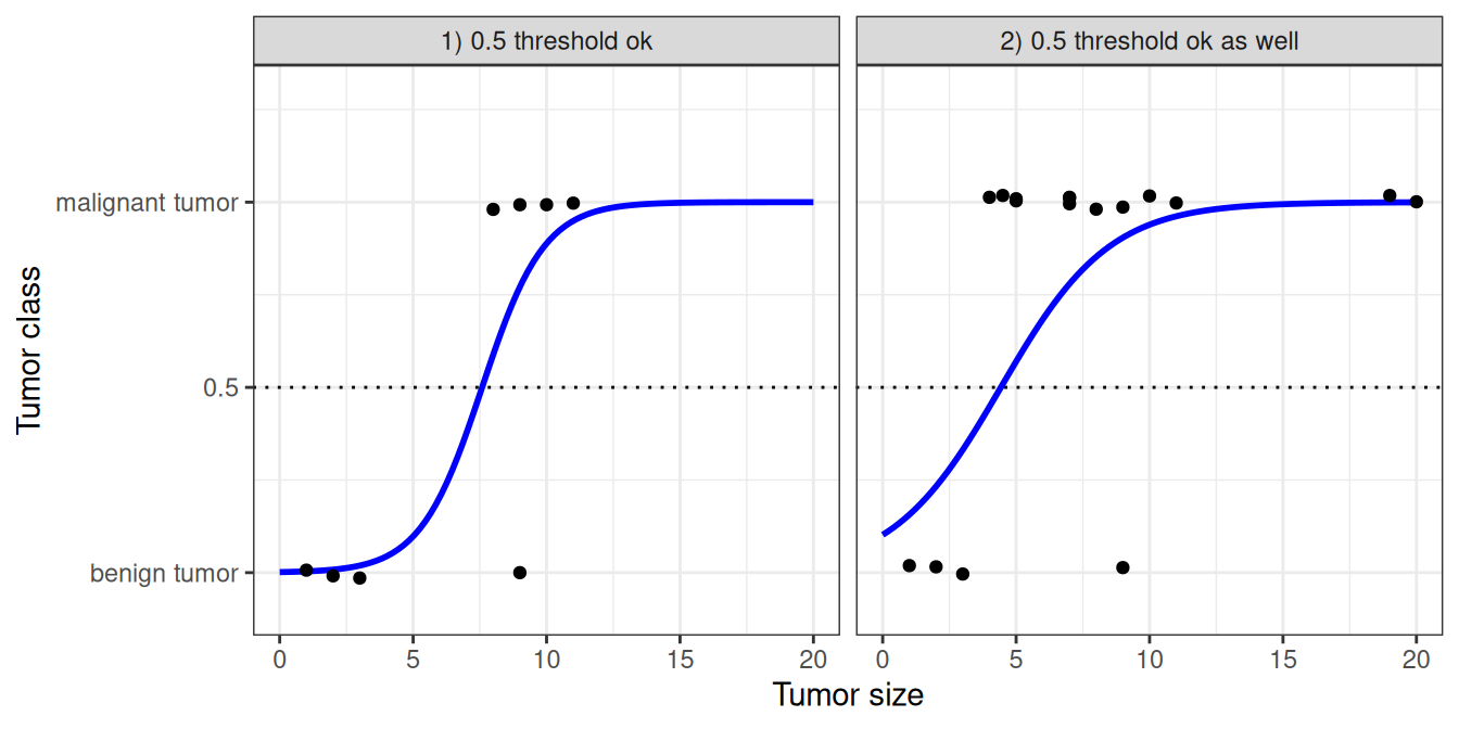
Classification works better with logistic regression, and we can use 0.5 as a threshold in both cases. The inclusion of additional points doesn’t really affect the estimated curve.
Interpretation
The interpretation of the weights in logistic regression differs from the interpretation of the weights in linear regression since the outcome in logistic regression is a value between 0 and 1. The weights don’t influence the probability linearly any longer. To interpret the weights, we need to reformulate the equation for the interpretation so that only the linear term is on the right side of the formula.
\[\ln\left(\frac{\mathbb{P}(Y=1)}{1-\mathbb{P}(Y=1)}\right)=\ln\left(\frac{\mathbb{P}(Y=1)}{\mathbb{P}(Y=0)}\right) = \beta_{0} + \beta_{1} x_{1} + \ldots + \beta_{p} x_{p}\]
We call the term in the ln() function “odds” (probability of event divided by probability of no event), and wrapped in the logarithm, it is called log odds.
This formula shows that the logistic regression model is a linear model for the log odds. Great! That doesn’t sound helpful!
Logistic regression is multiplicative
On the level of probabilities, logistic regression is not linear in the features. Meaning an increase by one unit in the features doesn’t increase the probability by \(\beta_j\), but rather changes the probability multiplicatively.
With a little shuffling of the terms, you can figure out how the prediction changes when one of the features \(X_j\) is changed by 1 unit. To do this, we can first apply the \(\exp\) function to both sides of the equation:
\[\frac{\mathbb{P}(Y=1)}{1 - \mathbb{P}(Y = 1)} = \text{odds}=\exp\left(\beta_{0} + \beta_{1} x_{1} + \ldots + \beta_{p} x_{p}\right)\]
Then we compare what happens when we increase one of the feature values by 1. But instead of looking at the difference, we look at the ratio of the two predictions:
\[\frac{\text{odds}_{x_j+1}}{\text{odds}_{x_j}}=\frac{\exp\left(\beta_{0}+\beta_{1}x_{1}+\ldots+\beta_{j}(x_{j}+1)+\ldots+\beta_{p}x_{p}\right)}{\exp\left(\beta_{0}+\beta_{1}x_{1}+\ldots+\beta_{j}x_{j}+\ldots+\beta_{p}x_{p}\right)}\]
We apply the following rule:
\[\frac{\exp(a)}{\exp(b)}=\exp(a-b)\]
And we remove many terms:
\[\frac{\text{odds}_{x_j+1}}{\text{odds}_{x_j}}=\exp\left(\beta_{j}(x_{j}+1)-\beta_{j}x_{j}\right)=\exp\left(\beta_j\right)\]
In the end, we have something as simple as \(\exp()\) of a feature weight. A change in a feature by one unit changes the odds ratio (multiplicative) by a factor of \(\exp(\beta_j)\). We could also interpret it this way: A change in \(x^{(i)}_j\) by one unit increases the log odds ratio by the value of the corresponding weight. Most people interpret the odds ratio because thinking about the \(\ln\) of something is known to be hard on the brain. Interpreting the odds ratio already requires some getting used to. For example, if you have odds of 2, it means that the probability for \(Y=1\) is twice as high as \(Y=0\). If you have a weight (log odds ratio) of 0.7, then increasing the respective feature by one unit multiplies the odds by \(\exp(0.7)\) (approximately 2), and the odds change to 4. But usually you do not deal with the odds and interpret the weights only as the odds ratios. Because for actually calculating the odds, you would need to set a value for each feature, which only makes sense if you want to look at one specific instance of your dataset.
These are the interpretations for the logistic regression model with different feature types:
- Numerical feature: If you increase the value of \(x^{(i)}_{j}\) by one unit, the estimated odds change by a factor of \(\exp(\beta_{j})\).
- Binary categorical feature: One of the two values of the feature is the reference category (in some languages, the one encoded in 0). Changing \(x^{(i)}_{j}\) from the reference category to the other category changes the estimated odds by a factor of \(\exp(\beta_{j})\).
- Categorical feature with more than two categories: One solution to deal with multiple categories is one-hot-encoding, meaning that each category has its own column. You only need L-1 columns for a categorical feature with L categories, otherwise it is over-parameterized. The L-th category is then the reference category. You can use any other encoding that can be used in linear regression. The interpretation for each category then is equivalent to the interpretation of binary features.
- Intercept \(\beta_{0}\): When all numerical features are zero and the categorical features are at the reference category, the estimated odds are \(\exp(\beta_{0})\). The interpretation of the intercept weight is usually not relevant.
Enhance interpretation with model-agnostic methods
If you want to interpret the outcome on the level of probabilities, then you have to use model-agnostic methods, such as the partial dependence plot.
Example
We use logistic regression to predict whether a penguin is female for Chinstrap penguins based on body measurements. The feature chonkiness is a discretization of the feature body_mass_g: Light penguins (0% to 25% quantile) are categorized as “Smol_Penguin”, most penguins are “Regular_Penguin”, and those with the highest body mass (75% to 100%) are categorized as “Absolute_Unit”. Normally, I don’t recommend discretizing continuous features because you lose information. In this case, I used binarization to illustrate the interpretation of a categorical feature with logistic regression, and I also love the word “chonky” and wanted to use it in a textbook.
Table 7.1 shows the estimated weights, associated odds ratios, and standard errors of the estimates.
| Weight | Std. Error | Odds ratio | |
|---|---|---|---|
| (Intercept) | 95.86 | 29.29 | 4.28931e+41 |
| bill_depth_mm | -2.06 | 0.83 | 0.13 |
| bill_length_mm | -0.53 | 0.19 | 0.59 |
| flipper_length_mm | -0.16 | 0.11 | 0.85 |
| chonkinessRegular_Penguin | 0.65 | 1.25 | 1.92 |
| chonkinessAbsolute_Unit | -0.84 | 1.66 | 0.43 |
Here are two examples of interpretation:
Numerical feature: An increase in a penguin’s bill length increases the odds of being female vs. male by a factor of 0.59 , when all other features remain the same.
Categorical feature: For the penguins of regular chonkiness, the odds of being female versus male are increased by a factor of 1.92 compared to lightweight penguins, given all other features remain the same. For the chonkiest penguins, the odds of being female versus male are decreased by a factor of 0.43 compared to lightweight penguins, given all other features remain the same. Again, given all other features remain the same.
The intercept is a very large value. This is because it is to be interpreted as odds of being female when all numerical features are set to zero and all categorical features are set to the reference level. This would be a non-chonky penguin with flipper length, bill length, and depth all at zero – not a realistic penguin. You could standardize the features, then the intercept would be more meaningful, but you can also just ignore the intercept.
Strengths
Many of the pros and cons of the linear regression model also apply to the logistic regression model.
On the good side, the logistic regression model is not only a classification model, but also gives you probabilities. This is a big advantage over models that can only provide the final classification. Knowing that an instance has a 99% probability for a class compared to 51% makes a big difference. However, you should check whether the probabilities are calibrated, meaning whether 60% really means 60%.
Logistic regression can also be extended from binary classification to multi-class classification.
Limitations
Logistic regression has been widely used by many different people, but it struggles with its restrictive expressiveness (e.g., interactions must be added manually), and other models may have better predictive performance.
Another disadvantage of the logistic regression model is that the interpretation is more difficult because the interpretation of the weights is multiplicative and not additive.
Logistic regression can suffer from complete separation. If there is a feature that would perfectly separate the two classes, the logistic regression model can no longer be trained. This is because the weight for that feature would not converge, because the optimal weight would be infinite. This is really a bit unfortunate because such a feature is really useful. But you do not need machine learning if you have a simple rule that separates both classes. The problem of complete separation can be solved by introducing penalization of the weights or defining a prior probability distribution of weights.
Software
I used the glm function in R for all examples. You can find logistic regression in any programming language that can be used for performing data analysis, such as Python, Java, Stata, Matlab, …
To be accurate, logistic regression is a regression model, since the output is continuous. But together with a decision threshold, like 0.5, it can be used for classification as well.↩︎