18 SHAP
SHAP (SHapley Additive exPlanations) by Lundberg and Lee (2017) is a method to explain individual predictions. SHAP is based on the game-theoretically optimal Shapley values. I recommend reading the chapter on Shapley values first.
To understand why SHAP is a thing and not just an extension of the Shapley values chapter, a bit of history: In 1953, Lloyd Shapley introduced the concept of Shapley values for game theory. Shapley values for explaining machine learning predictions were suggested for the first time by Štrumbelj and Kononenko (2011) and Štrumbelj and Kononenko (2014). However, they didn’t become so popular. A few years later, Lundberg and Lee (2017) proposed SHAP, which was basically a new way to estimate Shapley values for interpreting machine learning predictions, along with a theory connecting Shapley values with LIME and other post-hoc attribution methods, and a bit of additional theory on Shapley values.
You might say that SHAP is just a rebranding of Shapley values (which is true), but that would miss the fact that SHAP also marks a change in popularity and usage of Shapley values, and introduced new ways of estimating Shapley values and aggregating them in new ways. Also, SHAP brought Shapley values to text and image models.
While this chapter could totally be a subchapter of the Shapley value chapter, you can also see it as Shapley values 2.0 for interpreting machine learning models. This chapter emphasizes the new ways to estimate Shapley values and the new types of plots. But first, a bit of theory.
Tip
Looking for a comprehensive, hands-on guide to SHAP and Shapley values? Interpreting Machine Learning Models with SHAP has you covered. With practical Python examples using the shap package, you’ll learn how to explain models ranging from simple to complex. It dives deep into the mechanics of SHAP, provides interpretation templates, and highlights key limitations, giving you the insights you need to apply SHAP confidently and effectively.
SHAP theory
The goal of SHAP is to explain the prediction of an instance \(\mathbf{x}\) by computing the contribution of each feature to the prediction. SHAP computes Shapley values from coalitional game theory, the same as we discussed in the Shapley value chapter. The feature values of a data instance act as players in a coalition. Shapley values tell us how to fairly distribute the “payout” (= the prediction) among the features. A player can be an individual feature value, e.g., for tabular data. A player can also be a group of feature values. For example, to explain an image, pixels can be grouped into superpixels, and the prediction distributed among them. One innovation that SHAP brings to the table is that the Shapley value explanation is represented as an additive feature attribution method, a linear model. That view connects LIME and Shapley values. SHAP specifies the explanation as:
\[g(\mathbf{z}')=\phi_0+\sum_{j=1}^M\phi_j z_j'\]
where \(g\) is the explanation model, \(\mathbf{z}' = (z_1', \ldots, z_M')^T \in \{0,1\}^M\) is the coalition vector, \(M\) is the maximum coalition size, and \(\phi_j \in \mathbb{R}\) is the feature attribution for feature \(j\), the Shapley values. What I call “coalition vector” is called “simplified features” in the SHAP paper. I think this name was chosen because, for e.g., image data, the images are not represented on the pixel level, but aggregated into superpixels. It’s helpful to think about the \(\mathbf{z}'\) as describing coalitions: In the coalition vector, an entry of 1 means that the corresponding feature value is “present” and 0 that it is “absent”. But again, a feature here can be different from features the model used, like superpixels instead of pixels. The important part is that we can map between the two representations. To compute Shapley values, we simulate that only some feature values are playing (“present”) and some are not (“absent”). The representation as a linear model of coalitions is a trick for the computation of the \(\phi_j\)’s. For \(\mathbf{x}\), the instance of interest, the coalition vector \(\mathbf{x}'\) is a vector of all 1’s, i.e. all feature values are “present”. The formula simplifies to:
\[g(\mathbf{x}')=\phi_0+\sum_{j=1}^M\phi_j\]
You can find this formula in similar notation in the Shapley value chapter. More about the actual estimation comes later in this chapter. Let’s first talk about the properties of the \(\phi\)’s before we go into the details of their estimation.
Shapley values are the only solution that satisfies properties of Efficiency, Symmetry, Dummy, and Additivity. SHAP also satisfies these since it computes Shapley values. In the SHAP paper by Lundberg and Lee (2017), you will find discrepancies between SHAP properties and Shapley properties. SHAP describes the following three desirable properties:
1) Local accuracy
\[\hat{f}(\mathbf{x})=g(\mathbf{x}')=\phi_0+\sum_{j=1}^M\phi_j x_j'\]
If you define \(\phi_0=\mathbb{E}[\hat{f}(X)]\) and set all \(x_j'\) to 1, this is the Shapley efficiency property. Only with a different name and using the coalition vector.
\[\hat{f}(\mathbf{x}) = \phi_0 + \sum_{j=1}^M \phi_j x_j' = \mathbb{E}[\hat{f}(X)] + \sum_{j=1}^M\phi_j\]
2) Missingness
\[x_j'=0 \Rightarrow \phi_j=0\]
Missingness says that a missing feature gets an attribution of zero. Note that \(x_j'\) refers to the coalitions where a value of 0 represents the absence of a feature value. In coalition notation, all feature values \(x_j'\) of the instance to be explained should be ‘1’. This property is not among the properties of the “normal” Shapley values. So why do we need it for SHAP? Lundberg calls it a “minor book-keeping property”. A missing feature could – in theory – have an arbitrary Shapley value without hurting the local accuracy property, since it is multiplied with \(x_j'=0\). The Missingness property enforces that missing features get a Shapley value of 0. In practice, this is only relevant for features that are constant.
3) Consistency
Let \(\hat{f}_\mathbf{x}(\mathbf{z}') = \hat{f}(h_\mathbf{x}(\mathbf{z}'))\) and \(\mathbf{z}_{-j}'\) indicate that \(z_j'=0\). For any two models \(\hat{f}\) and \(\hat{f}'\) that satisfy:
\[\hat{f}_\mathbf{x}^{\prime}(\mathbf{z}') - \hat{f}_\mathbf{x}'(\mathbf{z}_{-j}') \geq \hat{f}_\mathbf{x}(\mathbf{z}') - \hat{f}_\mathbf{x}(\mathbf{z}_{-j}')\]
for all inputs \(\mathbf{z}'\in\{0,1\}^M\), then:
\[\phi_j(\hat{f}', \mathbf{x}) \geq \phi_j (\hat{f}, \mathbf{x})\]
The notation \(\phi_j(\hat{f}, \mathbf{x})\) emphasizes which model and data point the Shapley values depend on. The consistency property says that if a model changes so that the marginal contribution of a feature value increases or stays the same (regardless of other features), the Shapley value also increases or stays the same. From Consistency, the Shapley properties Linearity, Dummy, and Symmetry follow, as described in the Supplemental of Lundberg and Lee (2017).
SHAP estimation
This section is about three ways to estimate Shapley values for explaining predictions: KernelSHAP, Permutation Method, and TreeSHAP.
KernelSHAP
The situation with KernelSHAP is a bit confusing: It has been the entire motivation for SHAP, linked it with LIME and other attribution methods, and was introduced in the original paper Lundberg and Lee (2017). Also, many blog posts and so on about SHAP talk about KernelSHAP. But KernelSHAP is slow compared to TreeSHAP and the Permutation Method, and that’s why the shap Python package no longer uses it. Even if no longer the default, KernelSHAP helps to understand Shapley values and shows how Shapley values and LIME are connected, and some implementations still use it.
The KernelSHAP estimation has five steps:
- Sample coalition vectors \(\mathbf{z}_k' \in \{0,1\}^M, \quad k \in \{1,\ldots,K\}\) (1 = feature present in coalition, 0 = feature absent).
- Get prediction for each \(\mathbf{z}_k'\) by first converting \(\mathbf{z}_k'\) to the original feature space and then applying model \(\hat{f}: \hat{f}(h_{\mathbf{x}}(\mathbf{z}_k'))\).
- Compute the weight for each coalition \(\mathbf{z}_k'\) with the SHAP kernel.
- Fit weighted linear model.
- Return Shapley values \(\phi_k\), the coefficients from the linear model.
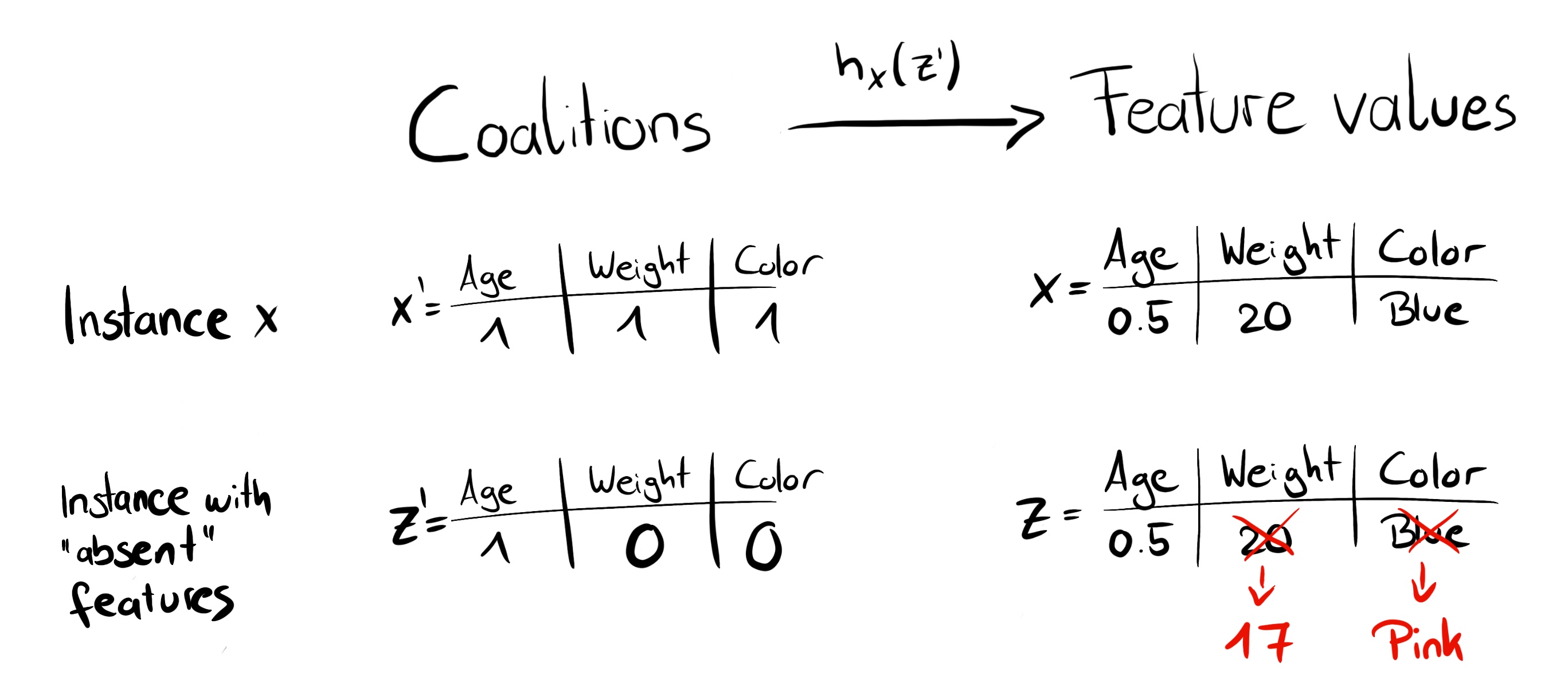
We can create a random coalition by repeated coin flips until we have a chain of 0’s and 1’s. For example, the vector of \((1,0,1,0)^T\) means that we have a coalition of the first and third features. The \(K\) sampled coalitions become the dataset for the regression model. The target for the regression model is the prediction for a coalition. (“Hold on!,” you say. “The model has not been trained on these binary coalition data and cannot make predictions for them.”) To get from coalitions of feature values to valid data instances, we need a function \(h_\mathbf{x}(\mathbf{z}') = \mathbf{z}\) where \(h_\mathbf{x}: \{0,1\}^M\rightarrow\mathbb{R}^p\). The function \(h_\mathbf{x}\) maps 1’s to the corresponding value from the instance \(\mathbf{x}\) that we want to explain. For tabular data, it maps 0’s to the values of another instance that we sample from the data. This means that we equate “feature value is absent” with “feature value is replaced by random feature value from data”. For tabular data, Figure 18.1 visualizes the mapping from coalitions to feature values.
\(h_{\mathbf{x}}\) for tabular data treats feature \(X_j\) and \(X_{-j}\) (the other features) as independent and integrates over the marginal distribution:
\[\hat{f}(h_{\mathbf{x}}(\mathbf{z}')) = \mathbb{E}_{X_{-j}}[\hat{f}(x_j, X_{-j})]\]
Sampling from the marginal distribution means ignoring the dependence structure between present and absent features. KernelSHAP therefore suffers from the same problem as all permutation-based interpretation methods. The estimation potentially puts weight on unlikely instances. Results can become unreliable. Would we sample from the conditional distribution, the value function would change, and therefore the game to which Shapley values are the solution. As a result, the Shapley values have a different interpretation: For example, a feature that might not have been used by the model at all can have a non-zero Shapley value when the conditional sampling is used. For the marginal game, this feature value would always get a Shapley value of 0, because otherwise it would violate the Dummy axiom. This conditional sampling version of SHAP exists and was suggested by Aas, Jullum, and Løland (2021).
Conditional Shapley values may give non-zero Shapley values to unused features
The problem with the conditional expectation is that features that have no influence on the prediction function \(\hat{f}\) can get a TreeSHAP estimate different from zero, as shown by Sundararajan and Najmi (2020) and Janzing, Minorics, and Blöbaum (2020). The non-zero estimate can happen when the feature is correlated with another feature that actually has an influence on the prediction.
For images, Figure 18.2 describes a possible mapping function. Assigning the average color of surrounding pixels or similar would also be an option.
The big difference between SHAP and LIME is the weighting of the instances in the regression model. LIME weights the instances according to how close they are to the original instance. The more 0’s in the coalition vector, the smaller the weight in LIME. SHAP weights the sampled instances according to the weight the coalition would get in the Shapley value estimation. Small coalitions (few 1’s) and large coalitions (i.e. many 1’s) get the largest weights. The intuition behind it is: We learn most about individual features if we can study their effects in isolation. If a coalition consists of a single feature, we can learn about this feature’s isolated main effect on the prediction. If a coalition consists of all but one feature, we can learn about this feature’s total effect (main effect plus feature interactions). If a coalition consists of half the features, we learn little about an individual feature’s contribution, as there are many possible coalitions with half of the features. To achieve Shapley compliant weighting, Lundberg and Lee (2017) proposed the SHAP kernel:
\[\pi_{\mathbf{x}}(\mathbf{z}') = \frac{(M-1)}{\binom{M}{|\mathbf{z}'|} |\mathbf{z}'| (M - |\mathbf{z}'|)}\]
Here, \(M\) is the maximum coalition size and \(|\mathbf{z}'|\) the number of present features in instance \(\mathbf{z}'\). Lundberg and Lee (2017) show that linear regression with this kernel weight yields Shapley values. If you were to use the SHAP kernel with LIME on the coalition data, LIME would also estimate Shapley values!
We can be a bit smarter about the sampling of coalitions: The smallest and largest coalitions take up most of the weight. We get better Shapley value estimates by using some of the sampling budget \(K\) to include these high-weight coalitions instead of sampling blindly. We start with all possible coalitions with 1 and \(M-1\) features, which makes \(2M\) coalitions in total. When we have enough budget left (current budget is \(K - 2M\)), we can include coalitions with 2 features and with \(M-2\) features and so on. From the remaining coalition sizes, we sample with readjusted weights.
We have the data, the target and the weights; Everything we need to build our weighted linear regression model:
\[g(\mathbf{z}') = \phi_0 + \sum_{j=1}^M \phi_j z_j'\]
We train the linear model \(g\) by optimizing the following loss function \(L\):
\[L(\hat{f}, g, \pi_{\mathbf{x}}) = \sum_{\mathbf{z}' \in \mathbf{Z}} [\hat{f}(h_{\mathbf{x}}(\mathbf{z}')) - g(\mathbf{z}')]^2 \pi_{\mathbf{x}}(\mathbf{z}')\]
where \(\mathbf{Z}\) is the training data. This is the good old boring sum of squared errors that we usually optimize for linear models. The estimated coefficients of the model, the \(\phi_j\)’s, are the Shapley values.
Since we are in a linear regression setting, we can also make use of the standard tools for regression. For example, we can add regularization terms to make the model sparse. If we add an L1 penalty to the loss \(L\), we can create sparse explanations. (I’m not so sure whether the resulting coefficients would still be valid Shapley values though.)
TreeSHAP
Lundberg, Erion, and Lee (2019) proposed TreeSHAP, a variant of SHAP for tree-based machine learning models such as decision trees, random forests, and gradient-boosted trees. TreeSHAP was introduced as a fast, model-specific alternative to KernelSHAP. How much faster is TreeSHAP? Compared to exact KernelSHAP, it reduces the computational complexity from \(O(TL2^M)\) to \(O(TLD^2)\), where T is the number of trees, L is the maximum number of leaves in any tree, and D is the maximal depth of any tree.
TreeSHAP comes in two versions:
- “Interventional” computes the classic Shapley values.
- “Tree-path dependent” computes something akin to conditional SHAP values.
The original implementation in the shap Python package used to be the tree-path dependent version, but is now the interventional one.
The estimation for both interventional and tree-path dependent estimation is rather complex, so I’ll just give you the rough idea (read: I haven’t fully understood the full version myself). Essentially, TreeSHAP leverages the tree structure to compute the Shapley values more efficiently.
Interventional TreeSHAP calculates the usual SHAP values. The following description is for estimating Shapley values for a single tree, for a data point \(\mathbf{x}\) to explain, and, for simplicity, the background dataset contains just one data point \(\mathbf{z}\):
The Shapley value, as we know, is computed by repeatedly forming coalitions of feature values, which includes present players (feature values from \(\mathbf{x}\)) and absent players (feature values from \(\mathbf{z}\)). However, for many of these coalitions, adding a feature from \(\mathbf{x}\) wouldn’t change the prediction, since a decision tree only has a limited amount of distinct predictions due to the decision structure. For example, a binary tree of depth 5 has a maximum of 32 possible predictions. So instead of iterating through all coalitions, the Interventional TreeSHAP estimator explores the tree paths to only work with the coalitions that would actually change the predictions. The tricky part is to correctly weight and combine these marginal contributions, which makes the interventional TreeSHAP algorithm more difficult to understand. And of course, damn recursion. To get the Shapley values for an ensemble of trees, for example for a random forest, simply combine the Shapley values the same way the ensemble predictions are combined. In the case of a random forest, it would be averaging the values.
Path-dependent TreeSHAP works in a similar fashion, making use of the tree structure. The basic idea is to push all subsets of coalition S down the tree simultaneously. And in each split, we keep track of the number of instances for the subsets.
Permutation Method
The most efficient model-agnostic estimator is the Permutation Method. The idea is to sample cleverly from the coalitions by creating permutations of the features.
Let’s look at an example (taken from the book Interpreting Machine Learning Models with SHAP) with four feature values: \(x_{\text{park}}, x_{\text{cat}}, x_{\text{area}}\), and \(x_{\text{floor}}\). For simplicity, I’ll shorten \(x^{(i)}_{\text{park}}\) as \(x_{\text{park}}\).
A random permutation of these features would be:
\[(x_{\text{cat}}, x_{\text{area}}, x_{\text{park}}, x_{\text{floor}})\]
Based on this permutation, we can compute marginal contributions by starting to build coalitions from left to right:
- Add \(x_{\text{cat}}\) to \(\emptyset\)
- Add \(x_{\text{area}}\) to \(\{x_{\text{cat}}\}\)
- Add \(x_{\text{park}}\) to \(\{x_{\text{cat}}, x_{\text{area}}\}\)
- Add \(x_{\text{floor}}\) to \(\{x_{\text{cat}}, x_{\text{area}}, x_{\text{park}}\}\)
And the same we can do backwards:
- Add \(x_{\text{floor}}\) to \(\emptyset\)
- Add \(x_{\text{park}}\) to \(\{x_{\text{floor}}\}\)
- Add \(x_{\text{area}}\) to \(\{x_{\text{park}}, x_{\text{floor}}\}\)
- Add \(x_{\text{cat}}\) to \(\{x_{\text{area}}, x_{\text{park}}, x_{\text{floor}}\}\)
The permutation changes one feature at a time. This reduces the number of model calls since the second term of a marginal contribution (a model prediction) is also needed to compute the next marginal contribution. For example, the coalition \(\{x_{\text{cat}}, x_{\text{area}}\}\) is used to calculate both the marginal contribution of \(x_{\text{park}}\) to \(\{x_{\text{cat}}, x_{\text{area}}\}\) and of \(x_{\text{area}}\) to \(\{x_{\text{cat}}\}\). Each forward and backward permutation gives us two marginal contributions per feature. By doing a couple of permutations like this, we get a pretty good estimate of the Shapley values. To actually compute the Shapley values, we have to define the Shapley values in terms of permutations instead of coalitions: There are \(p!\) possible permutations of the features and \(o(k)\) the k-th permutation, then the Shapley value for feature \(j\) can be computed as:
\[\hat{\phi}_j^{(i)} = \frac{1}{m} \sum_{k=1}^m \hat{\Delta}_{o(k), j}\]
The term \(\hat{\Delta}_{o(k), j}\) is the \(k\)-th marginal contribution. This means we can compute the Shapley value as a simple average over all contributions. However, the motivation for permutation estimation was to avoid computing all possible coalitions or permutations. Good thing is we can sample permutations and still take the average. Since we perform forward and backward iterations, we compute the Shapley value as:
\[\hat{\phi}_j^{(i)} = \frac{1}{2m} \sum_{k=1}^m (\hat{\Delta}_{o(k), j} + \hat{\Delta}_{-o(k), j})\]
Permutation \(-o(k)\) is the reverse version of the permutation. The permutation procedure with forward and backward iterations, also known as antithetic sampling, performs quite well compared to other SHAP value sampling estimators (Mitchell et al. 2022). The permutation method additionally ensures that the efficiency axiom is always satisfied, meaning when you add up the SHAP values, they equal prediction minus average prediction. For a rough idea of how many permutations you might need: the shap package defaults to 10.
Example
I trained a random forest classifier with 100 trees to predict the penguin sex. We’ll use SHAP to explain individual predictions. We can use the fast Interventional TreeSHAP estimation method instead of the slower KernelSHAP method, since a random forest is an ensemble of trees. But instead of relying on the conditional distribution, this example uses the marginal distribution. This is described in the package, but not in the original paper. The Python TreeSHAP function is slower with the marginal distribution, but still faster than KernelSHAP, since it scales linearly with the rows in the data.
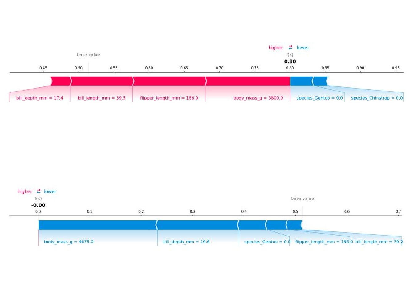
Because we use the marginal distribution here, the interpretation is the same as in the Shapley value chapter. But with the Python shap package comes a different visualization: You can visualize feature attributions such as Shapley values as “forces.” Each feature value is a force that either increases or decreases the prediction. The prediction starts from the baseline. The baseline for Shapley values is the average of all predictions. In the plot, each Shapley value is an arrow that pushes to increase (positive value) or decrease (negative value) the prediction. These forces balance each other out at the actual prediction of the data instance.
Tip
The shap Python package comes with a lot of different visualizations, which can be confusing. That’s why I summarized them in this SHAP Plots Cheatsheet, along with how to interpret the plots.
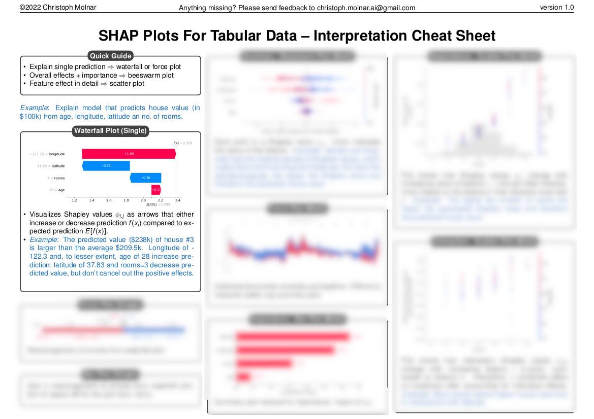
Figure 18.3 shows SHAP explanation force plots for two penguins from the Palmer penguins dataset: The first penguin has a high probability of being an Adelie penguin due to its small bill length. The second penguin is unlikely to be Adelie due to its large bill length and flipper length.
SHAP aggregation plots
The section before showed explanations for individual predictions.
Shapley values can be combined into global explanations. If we run SHAP for every instance, we get a matrix of Shapley values. This matrix has one row per data instance and one column per feature. We can interpret the entire model by analyzing the Shapley values in this matrix.
We start with SHAP feature importance.
SHAP Feature Importance
The idea behind SHAP feature importance is simple: Features with large absolute Shapley values are important. Since we want the global importance, we average the absolute Shapley values per feature across the data:
\[I_j=\frac{1}{n}\sum_{i=1}^n |\phi_j^{(i)}|\]
Next, we sort the features by decreasing importance and plot them. Figure 18.4 shows the SHAP feature importance for the random forest trained before for classifying penguins. The body mass was the most important feature, changing the predicted probability for Adelie 25 percentage points (0.25 on the x-axis).
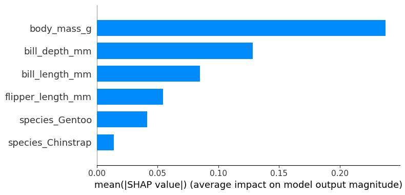
SHAP feature importance is an alternative to permutation feature importance. There’s a big difference between both importance measures: Permutation feature importance is based on the decrease in model performance. SHAP is based on the magnitude of feature attributions.
The feature importance plot is useful, but contains no information beyond the importances. For a more informative plot, we will next look at the summary plot.
SHAP Summary Plot
The summary plot combines feature importance with feature effects. Each point on the summary plot is a Shapley value for a feature and an instance. The position on the y-axis is determined by the feature and on the x-axis by the Shapley value. The color represents the value of the feature from low to high. Overlapping points are jittered in the y-axis direction, so we get a sense of the distribution of the Shapley values per feature. The features are ordered according to their importance. In the summary plot, Figure 18.5, we see first indications of the relationship between the value of a feature and the impact on the prediction. A higher body mass contributes negatively to P(female). The summary plot also shows that body mass has the widest range of effects for the different penguins.
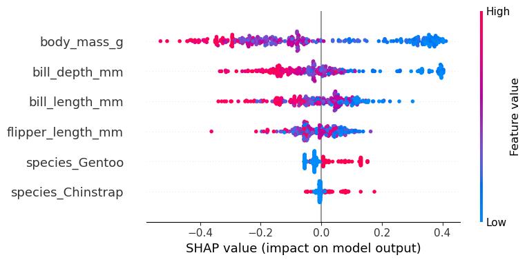
But to see the exact form of the relationship, we have to look at SHAP dependence plots.
SHAP Dependence Plot
SHAP feature dependence might be the simplest global interpretation plot: 1) Pick a feature. 2) For each data instance, plot a point with the feature value on the x-axis and the corresponding Shapley value on the y-axis. 3) Done.
Mathematically, the plot contains the following points: \(\{(x_j^{(i)}, \phi_j^{(i)})\}_{i=1}^n\)
Figure 18.6 shows the SHAP feature dependence for the body mass. The heavier the penguin, the less likely it’s female.
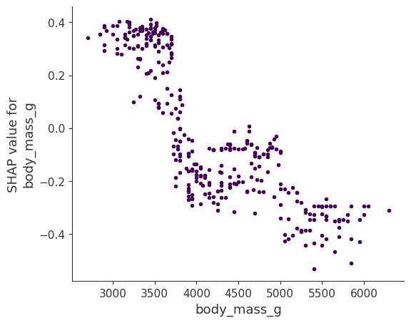
SHAP dependence plots are an alternative to global feature effect methods like the partial dependence plots and accumulated local effects. While PDP and ALE plots show average effects, SHAP dependence also shows the variance on the y-axis. Especially in the case of interactions, the SHAP dependence plot will be much more dispersed on the y-axis. The dependence plot can be improved by highlighting these feature interactions.
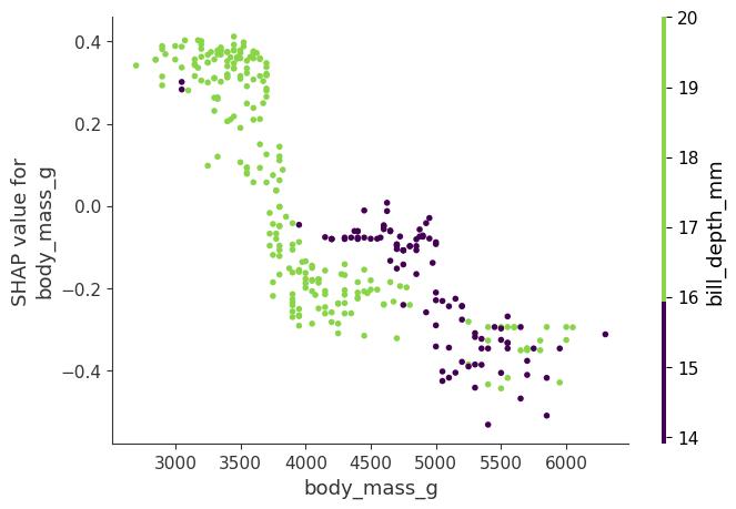
SHAP Interaction Values
The interaction effect is the additional combined feature effect after accounting for the individual feature effects. The Shapley interaction index from game theory is defined as:
\[\phi_{i,j}=\sum_{S\subseteq\backslash\{i,j\}}\frac{|S|!(M-|S|-2)!}{2(M-1)!}\delta_{ij}(S)\]
when \(i\neq{}j\) and \(\delta_{ij}(S)=\hat{f}_{\mathbf{x}}(S\cup\{i,j\})-\hat{f}_{\mathbf{x}}(S\cup\{i\})-\hat{f}_{\mathbf{x}}(S\cup\{j\})+\hat{f}_{\mathbf{x}}(S)\).
This formula subtracts the main effect of the features so that we get the pure interaction effect after accounting for the individual effects. We average the values over all possible feature coalitions \(S\), as in the Shapley value computation. When we compute SHAP interaction values for all features, we get one matrix per instance with dimensions \(M \times M\), where \(M\) is the number of features. How can we use the interaction index? For example, to automatically color the SHAP feature dependence plot with the strongest interaction, as in Figure 18.7. Here, body mass interacts with bill depth.
Analyze interactions in depth
The topic of SHAP and interactions goes a lot deeper. If you require more sophisticated analysis of SHAP interactions, I recommend looking into the shapiq package (Muschalik et al. 2024).
Clustering Shapley Values
You can cluster your data with the help of Shapley values. The goal of clustering is to find groups of similar instances. Normally, clustering is based on features. Features are often on different scales. For example, height might be measured in meters, color intensity from 0 to 100, and some sensor output between -1 and 1. The difficulty is to compute distances between instances with such different, non-comparable features.
SHAP clustering works by clustering the Shapley values of each instance. This means that you cluster instances by explanation similarity. All SHAP values have the same unit – the unit of the prediction space. You can use any clustering method.
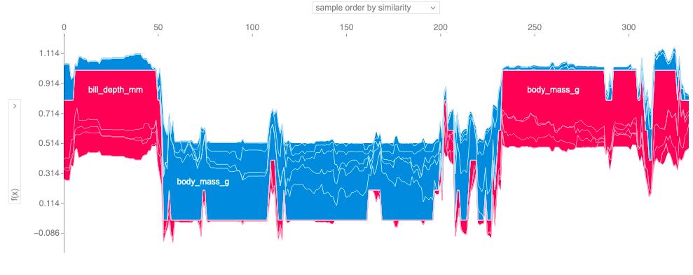
Figure 18.8 uses hierarchical agglomerative clustering to order the instances. The plot consists of many force plots, each of which explains the prediction of an instance. We rotate the force plots vertically and place them side by side according to their clustering similarity.
Strengths
Since SHAP computes Shapley values, all the advantages of Shapley values apply: SHAP has a solid theoretical foundation in game theory. The prediction is fairly distributed among the feature values. We get contrastive explanations that compare the prediction with the average prediction.
SHAP connects LIME and Shapley values. This is very useful to better understand both methods. It also helps to unify the field of interpretable machine learning.
SHAP has a fast implementation for tree-based models. I believe this was key to the popularity of SHAP because the biggest barrier for adoption of Shapley values is the slow computation.
The fast computation makes it possible to compute the many Shapley values needed for the global model interpretations. The global interpretation methods include feature importance, feature dependence, interactions, clustering, and summary plots. With SHAP, global interpretations are consistent with the local explanations, since the Shapley values are the “atomic unit” of the global interpretations. If you use LIME for local explanations and partial dependence plots plus permutation feature importance for global explanations, you lack a common foundation.
Limitations
KernelSHAP is slow. This makes KernelSHAP impractical to use when you want to compute Shapley values for many instances. Also, all global SHAP methods, such as SHAP feature importance, require computing Shapley values for a lot of instances.
KernelSHAP ignores feature dependence. Most other permutation-based interpretation methods have this problem. By replacing feature values with values from random instances, it is usually easier to randomly sample from the marginal distribution. However, if features are dependent, e.g., correlated, this leads to putting too much weight on unlikely data points.
Path-dependent TreeSHAP can produce unintuitive feature attributions. While TreeSHAP solves the problem of extrapolating to unlikely data points, it does so by changing the value function and therefore slightly changes the game. TreeSHAP changes the value function by relying on the conditional expected prediction. With the change in the value function, features that have no influence on the prediction can get a TreeSHAP value different from zero.
The disadvantages of Shapley values also apply to SHAP: Shapley values can be misinterpreted.
It’s possible to create intentionally misleading interpretations with SHAP, which can hide biases (Slack et al. 2020). If you are the data scientist creating the explanations, this is not an actual problem (it would even be an advantage if you are the evil data scientist who wants to create misleading explanations). For the receivers of a SHAP explanation, it’s a disadvantage: they cannot be sure about the truthfulness of the explanation.
Software
Lundberg implemented SHAP in the shap Python package, which is now maintained by a much bigger team.
This implementation works for models trained with the scikit-learn machine learning library for Python. The shap package was also used for the examples in this chapter. SHAP is integrated into the tree boosting frameworks xgboost and LightGBM, and you can find it in PiML, a more general interpretability library. In R, there are the shapper and fastshap packages. SHAP is also included in the R xgboost package. Specifically for SHAP interactions, there is the Python shapiq package.